Why Continuous TSS Replaced Turbidity-Only Stations
A suspended solids online monitoring system reports continuous TSS in mg/L every 1 second to 1 minute on industrial and municipal effluent. Permit limits use flow-averaged mg/L, not NTU. A stable 12 NTU turbidity trend can mask a 400 mg/L TSS violation for hours when the optical window fouls (per Olpas, 2025-05).
Storm inflow, clarifier upset, or polymer overfeed can double effluent TSS in under ten minutes. That spike arrives before any 24-hour composite sample is pulled (Olpas, 2025-05). Continuous mg/L output is the compliance baseline for discharge reporting in 2026. Turbidity-only stations are hard to defend in a regulator audit. Pair the analyzer with the layered philosophy in the wastewater SCADA alarm management guide so high-high TSS trips divert flow or shut polymer before the excursion leaves the plant.
What a Suspended Solids Online Monitoring System Measures
In practice, suspended solids online monitoring is a continuous in-process package — an in-line or in-tank probe plus a separate transmitter — that outputs TSS in mg/L. The output is 4-20 mA analog, Modbus RTU, or Profinet/Ethernet-IP, never NTU. Four sensing principles are in commercial use: optical backscatter (typically 90°/180° near-infrared), optical reflectance, ultrasonic attenuation, and gravimetric correlation via paired density and velocity measurement.
The transmitter is sold separately from the sensor. A Badger Meter Q46/88, a Sper Scientific digital online TSS meter, and an IQ SensorNet ViSolid ship as meter plus probe. Those parts must be ordered together to form a working system (per Sper Scientific ordering notes). Factory calibration is a starting point only. Site-specific correlation against APHA 2540 D lab TSS is required for any permit-bound measurement. A complete system usually includes a wiper, a flow cell, and mounting hardware. The HydropureWater dissolved air flotation system skid ships with a side-stream TSS loop pre-engineered for this purpose.
Comparing the Four Sensor Technologies for Industrial Effluent
Sensor selection is a matrix problem: range, optical behavior, fouling tolerance, and cost all change with the stream. Optical backscatter (typical Hach TSS sc, Solitax) is the workhorse for 0-1,500 mg/L clarifier overflows. It is sensitive to color and particle size, and the optical window fouls in 2-4 weeks without a wiper. Optical reflectance (WTW ViSolid, some Endress+Hauser variants) pushes the upper range to 40,000 mg/L. It is largely color-independent and ships with an integrated wiper, which is why it dominates activated-sludge MLSS and DAF float monitoring.
Ultrasonic attenuation is non-optical, so it is immune to color, coatings, and grease. It suits thickener underflow, DAF sludge, and oily petrochemical streams, but costs roughly 2-3× an optical probe. Gravimetric correlation is rare in effluent and is mostly used in primary sludge lines. Most plants we size for secondary effluent run at the lower end of the backscatter range and add a wiper from day one.
| Sensor principle | Measurement range (mg/L TSS) | Accuracy | Output signal | Cleaning method | Typical application | Relative cost (USD, 2026) |
|---|---|---|---|---|---|---|
| Optical backscatter (NIR, 90°/180°) | 0-1,500 | ±5% of reading or ±2 mg/L | 4-20 mA + Modbus RTU | Air-blow or wiper, every 1-7 days | Clarifier overflow, sand filter effluent | $3,500-6,000 |
| Optical reflectance | 0-40,000 | ±5% of reading | 4-20 mA + Modbus RTU/TCP | Integrated silicone wiper, automatic | MLSS in aeration basin, DAF float | $5,000-9,000 |
| Ultrasonic attenuation | 0-50,000 | ±3-5% of reading | 4-20 mA + Profinet or Ethernet/IP | Non-contact, wipe-clean only | Thickener underflow, oily/greasy streams | $8,000-14,000 |
| Gravimetric correlation | 1,000-100,000 | ±10% of reading | 4-20 mA + Modbus | Manual, monthly | Primary/digested sludge lines | $10,000-18,000 |
Ranges and accuracy values are typical manufacturer specifications and should be confirmed against the selected vendor's data sheet before specification sign-off.
Where to Mount the Probe: In-Pipe, In-Tank, or Side-Stream
Placement is a hydraulic decision, not a sensor decision. In-pipe insertion via a hot-tap ball valve gives the smallest footprint and a clean reading because pipe flow self-scours the optical window. Line velocity must stay in the 0.3-2 m/s window or the reading drifts: low velocity fouls, high velocity adds bubble noise. In-tank immersion with a rigid or float-mounted probe is the standard for aeration basins and equalization tanks. It is the easiest retrofit, but activated-sludge matrices need an automatic wiper at least once per 30 minutes.
A side-stream slip stream with a small sample pump and a flow cell is the most maintainable option for dirty, oily, or fibrous streams. Manual cleaning takes 30 seconds. The 10-15 second hydraulic lag is irrelevant at the 1-minute sampling rates these systems run. A GX series rotary mechanical bar screen upstream of the TSS loop will cut ragging failures on immersed probes by roughly 80% based on HydropureWater field data, 2026.
| Mounting location | Best for | Watch out for |
|---|---|---|
| In-pipe (hot-tap insertion) | Treated effluent, filtered water, clean process streams | Line velocity must stay 0.3-2 m/s; air entrainment causes noise |
| In-tank (immersion, rigid or float) | Aeration basin MLSS, equalization tanks, DAF cells | Fouling without wiper; baffles can create dead zones |
| Side-stream (slip stream + flow cell) | Dirty, oily, or fibrous streams; primary sludge; centrate | Adds 10-15 s lag; pump maintenance required every 6-12 months |
Do suspended solids affect PFAS polishing trains?
Suspended solids carry particle-bound organics into downstream polishing steps that many plants use for micropollutants such as PFAS. High TSS loads foul membranes, shorten carbon bed life, and create false low readings on some optical analyzers when the window coats. Keep clarifier or DAF effluent TSS inside the design band before the polishing train. Use continuous mg/L feedback — not NTU alone — so solids spikes are caught in minutes rather than after a composite sample.
How does a VFD inverter use TSS feedback?
A variable-frequency drive (inverter) on a polymer dosing pump or sludge recycle pump can close on the TSS tag when the analyzer outputs 4-20 mA or a networked mg/L value. Rising effluent TSS ramps polymer feed. Falling TSS backs the drive down to cut overfeed. Cycle times under 10 ms on Profinet or Ethernet/IP matter only when the TSS reading is inside that control loop. Keep at least two relay outputs for high-high diversion so the drive is not the sole trip path.
Wiring and SCADA Integration: 4-20 mA, Modbus, and Profinet
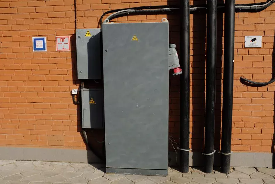
Specify a 4-20 mA passive (loop-powered) output as the baseline. Every legacy PLC and chart recorder speaks it, and the loop carries both signal and power on a single twisted pair. Layer Modbus RTU over RS-485 on the same analyzer for multi-drop networks. Modbus lets the SCADA log the actual mg/L value plus diagnostic flags (fouled window, wiper fault, out-of-range) that a 4-20 mA loop cannot convey. It also allows up to 32 analyzers on one trunk with 1,200 m cable reach.
For Industry 4.0 plants, Profinet or Ethernet/IP on newer analyzers maps the TSS tag directly into the PLC without a gateway. Speeds reach 100 Mbit with cycle times under 10 ms when the TSS reading closes a polymer feed loop. Plan for at least two relay outputs (SPDT, 5 A, 250 VAC) for high-high TSS alarms. A clarifier upset can then trigger automatic polymer shutdown or effluent diversion through the HydropureWater automatic chemical dosing skid. For the alarm-rationalization workflow on the SCADA side, follow the layered philosophy in the wastewater SCADA alarm management guide — one operational alarm, one safety alarm, one maintenance alarm per analyzer, no more.
Calibration Protocol: 1-Point, Multi-Point, and Site Correlation
Factory calibration is a marketing number, not a compliance number. For any TSS reading that will be reported against a discharge permit, a site-specific correlation against APHA 2540 D lab TSS is required. The procedure has four steps:
- Collect 10-15 paired samples across the normal operating range of the stream (low, normal, high, upset) over 2-3 weeks.
- Run each sample through APHA 2540 D in duplicate and average the result.
- Perform a linear regression (mg/L lab vs. mA or Modbus raw value) and load the slope and offset into the transmitter.
- Verify with a 2-point standard after every membrane, wiper, or lamp replacement — formazin works for low range, site-sourced supernatant for high range.
Recalibrate quarterly as a minimum, and always after any process change — new coagulant chemistry, a changed sludge age, or a new DAF unit. A documented calibration logbook with dates, paired data, regression coefficients, and the technician's signature is the artifact a regulator will ask for during an audit.
Cost-Per-Measurement: Online TSS vs Laboratory TSS
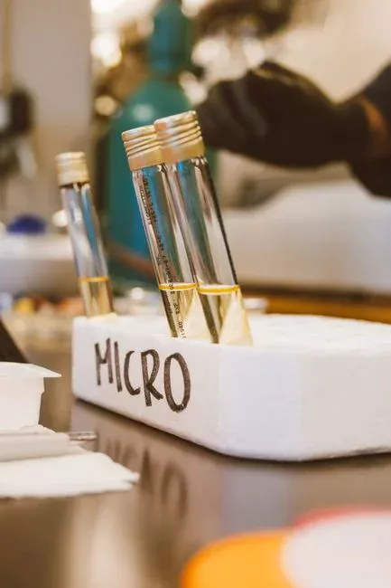
Lab TSS by APHA 2540 D runs $20-50 per sample in reagent and technician time. The 2-4 hour turnaround makes the result useless for real-time control. A continuous online analyzer at one reading per minute produces 1,440 measurements per day. Once CAPEX is amortized, the all-in cost is a few dollars per day. Payback on lab cost alone is 6-18 months at any plant running daily TSS.
Add the avoided-violation value: a single EPA effluent violation for an unreported TSS excursion commonly runs into five figures. The online lead analyzer buyer's guide covers a similar CAPEX-defensible math for metals. Plan for a 10-15 business day delivery lead time on imported inline analyzers (per Sper Scientific ordering notes) when you build the project schedule.
| Method | Measurements per day | Cost per measurement (USD, 2026) | Result latency | Permit-defensible? |
|---|---|---|---|---|
| Online TSS analyzer (1/min) | 1,440 | $0.01-0.05 (amortized) | < 1 minute | Yes, with site correlation |
| Online turbidity probe (NTU) | 1,440 | $0.01-0.05 (amortized) | < 1 minute | No — reports NTU, not mg/L TSS |
| Lab TSS, APHA 2540 D | 1 | $20-50 | 2-4 hours | Yes |
| Lab TSS, 24-hour composite | 1 | $40-80 | 24 hours | Yes (flow-weighted) |
Selection Checklist and Next Step
Who this is for: plant engineers, EPC instrument leads, and procurement managers specifying continuous TSS for NPDES or equivalent discharge reporting. Who should look elsewhere: teams that only need process turbidity for filter backwash timing and have no mg/L permit clause. Selection checklist before purchase:
- Confirm permit units are mg/L TSS and map the expected operating range (effluent vs MLSS vs sludge).
- Pick sensing principle for color, grease, and fouling — not for brochure range alone.
- Choose mounting (in-pipe 0.3-2 m/s, in-tank with wiper, or side-stream flow cell).
- Require 4-20 mA plus Modbus or industrial Ethernet, and two high-high relays.
- Budget site correlation to APHA 2540 D at commissioning and quarterly re-checks.
- Include wiper or air-clean hardware and spare windows in the spare-parts list.
- Schedule 10-15 business day lead time for imported inline analyzers.
If you are sizing a clarifier, DAF, or dosing loop around continuous TSS, send the stream range and permit limit through the HydropureWater inquiry form. The probe, mounting, and SCADA tags can then be checked against the same hydraulic design.
Frequently Asked Questions
What is the difference between TSS and turbidity?
TSS (total suspended solids) is a gravimetric concentration in mg/L measured by APHA 2540 D. Turbidity is an optical property in NTU that correlates with TSS but is also affected by color, particle size, and shape. The same NTU value can represent very different mg/L values across matrices (per Olpas, 2025-05). Online TSS analyzers output mg/L; turbidity probes output NTU and are not a permit substitute without documented site correlation.
What measuring range do I need for effluent TSS?
Secondary effluent typically runs 5-100 mg/L with a permit limit of 30 mg/L. Primary clarifier overflow runs 200-800 mg/L. Activated-sludge MLSS runs 2,000-5,000 mg/L. DAF float and thickener underflow run 10,000-40,000 mg/L. Match the sensor principle and range to the stream, then leave headroom for upset peaks.
Which output signal should I specify?
Specify 4-20 mA passive as the baseline for every PLC and recorder. Add Modbus RTU over RS-485 for diagnostics and multi-drop networks of up to 32 analyzers with 1,200 m cable reach. Use Profinet or Ethernet/IP only when the PLC is Industry 4.0 and the TSS tag must close a control loop with cycle times under 10 ms.
How often should an online TSS analyzer be calibrated?
Site-correlate against APHA 2540 D at commissioning with 10-15 paired samples over 2-3 weeks. Re-verify quarterly and after any process change. Perform a 2-point check with formazin or site-sourced standard after every wiper or lamp replacement, and keep a signed calibration logbook for audits.
Does online TSS meet EPA, EU, and China GB discharge permit reporting requirements?
Online TSS with documented site correlation against APHA 2540 D is accepted by EPA NPDES programs, EU Industrial Emissions Directive monitoring, and China GB 18918-2002 / GB 3544-2008 reporting. The analyzer output is a continuous equivalent of the lab method, not a substitute for the lab method itself. Regulators still expect the paired lab data and calibration record.