A polymer dosing system for wastewater treatment prepares, dilutes, and meters polymer to build settleable flocs. Feed spans 0.1–500 L/h at 0.1–0.5% strength, mixing runs 300–1200 RPM, and controlled feed often reaches 92–97% TSS removal.
Core hardware includes a preparation tank, metering pump, static mixer, and PLC panel, with automation cutting chemical waste by up to 30% versus manual feed. Plants using this approach often reach 92–97% total suspended solids (TSS) removal, against 60–80% without polymer.
What Does a Polymer Dosing System for Wastewater Treatment Do?
A polymer dosing system prepares a dilute solution and meters it into wastewater so colloidal solids form settleable flocs. Typical feed is 0.1–500 L/h at 0.1–0.5% strength, with wetting and aging mixers between 300–1200 RPM. Plants that hold that window often report 92–97% TSS removal, against about 60–80% when no polymer is used.
According to 40 CFR 133.102, the secondary-treatment suspended-solids limit is a 30-day average of 30 mg/L. The same section sets a 7-day average of 45 mg/L and a 30-day average percent removal of no less than 85 percent. Effluent pH must stay within the limits of 6.0 to 9.0 unless the treatment works meets the listed exceptions.
Earlier drafts of this guide called 92–97% TSS removal an EPA 2024 benchmark. That percent is a plant result, not the permit floor of 30 mg/L and 85 percent removal. Steady dosing also supports discharge limits such as the EPA typical target of less than 30 mg/L TSS. Correct control supports 92–97% TSS removal, shorter filter-press cycles, and steadier compliance near that 30 mg/L TSS line.
Controlled dosing prepares and injects polymer solutions into wastewater so colloidal particles form settleable flocs. Specs usually cover 0.1–500 L/h feed rates, 0.1–0.5% dilute strength, and 300–1200 RPM mixing. Poor flocculation can raise annual operating cost by over $200,000 at a typical industrial plant. A food processing site generating 500 m³/day of high-organic wastewater may see effluent TSS above 150 mg/L without optimized polymer feed.
Sludge then resists dewatering, disposal costs climb, and permit risk rises. Polymers bridge colloidal particles (typically 1–1000 nm) into larger flocs (1–5 mm) that settle faster in clarifiers or capture more readily on filter presses. With controlled polymer feed, TSS removal commonly rises to 92–97%, versus 60–80% without polymer (industry benchmarks). Filter press cycle times can fall 30–50%, which raises throughput and lowers energy use.
Preventing overfeed can cut chemical use 10–20%. Call the injected stream polymer dosing water only after dilution, not while a neat liquid is still concentrated. Steady polymer dosing holds those flocs near the 1–5 mm band instead of a sticky blanket. Most plants we size for food waste run the dilute solution at about 0.2%, the lower half of the 0.1–0.5% window, because cold water makes a stronger batch hard to wet.
How the System Works: Step-by-Step Process Mechanics
The polymer preparation unit converts raw polymer into an active dilute solution, then meters that solution into the wastewater stream. Performance depends on selection, wetting, aging, dilution, injection, and controlled mixing before floc growth. Most plants we size for wet dry polymer for 1–2 minutes, then age it before any transfer to the feed pump.
- Step 1: Polymer Selection – Match chemistry to particle charge, pH, and composition. Anionic grades suit positively charged particles; cationic grades suit negatively charged organics, such as food-process solids; non-ionic grades suit neutral or variable charge. Typical dosage is 0.5–10 mg/L from jar testing.
- Step 2: Preparation (Wetting & Aging) – Dry or emulsion polymers need rapid wetting for 1–2 minutes at about 300 RPM to avoid "fish-eyes." Aging then runs 30–60 minutes near 100 RPM so chains uncoil and activate, as polymer supplier guidelines document.
- Step 3: Dilution – Concentrated liquids (for example 10–20%) are diluted to about 0.1–0.5%. That range supports uniform dispersion; overly strong feed causes local overfeed and weak flocs.
- Step 4: Dosing – A metering pump injects the dilute solution. Peristaltic pumps suit lower flows and gentle handling; diaphragm pumps suit higher pressure and flow. Rates span 0.1 L/h on pilot skids to over 500 L/h on large plants (per manufacturer specifications).
- Step 5: Mixing – Static or dynamic mixers distribute polymer at once. Static mixers create turbulence at G-values of 700–1000 s⁻¹. Dynamic agitators run about 300–1200 RPM for floc start and growth, as recommended by EPA 2023 guidelines for flocculation.
- Step 6: Flocculation – Gentle mixing in a flocculation chamber grows microflocs into stable macroflocs. Retention is typically 2–5 minutes so flocs enlarge without shear breakup.
| Process Step | Key Parameter | Typical Range/Value | Impact on Efficiency |
|---|---|---|---|
| Preparation (Wetting) | Mixing Speed | 300 RPM | Prevents "fish-eyes," ensures full hydration. |
| Preparation (Aging) | Mixing Speed | 100 RPM | Allows polymer chains to uncoil, maximizes activity. |
| Dilution | Concentration | 0.1–0.5% | Optimizes polymer activation and dispersion. |
| Dosing | Flow Rate | 0.1–500 L/h | Controls polymer dosage in wastewater. |
| Mixing (G-value) | Velocity Gradient | 700–1000 s⁻¹ | Balances floc initiation and shear forces. |
| Flocculation | Retention Time | 2–5 minutes | Allows microflocs to grow into stable macroflocs. |
Plants that need closed-loop chemical feed often specify an Automatic Chemical Dosing System with PLC control for these same preparation and metering steps.
What Are Automated Polymer Dosing System Specifications?
Automated polymer dosing system specifications cover tank volume, mixer speed, pump accuracy, pipe diameter, and the sensors that trim the dose. Procurement teams should judge a skid by tank materials, pump accuracy, mixer geometry, and sensor feedback. Those details set reliability under continuous industrial duty. A nameplate flow without a stated accuracy and pressure is not yet a specification.
- Polymer Preparation Tank: HDPE resists corrosion; 316 stainless steel suits hotter or harsher service. Capacities run from 50 L on compact skids to over 2000 L on large plants. Agitators typically wet at 300–1200 RPM, then age at 50–150 RPM. Cold sites may heat solution to 15–25°C to hold viscosity.
- Metering Pump: Flow spans 0.1–500 L/h with about ±1% accuracy under stable conditions and 1–10 bar pressure rating. Peristaltic designs protect shear-sensitive chains; diaphragm designs tolerate higher pressure and minor grit.
- Static Mixer: Pipe diameters of 25–150 mm with 6–12 elements disperse polymer fast. PVC fits general duty; 316 stainless steel fits aggressive chemistry. Pressure drop is often 0.1–0.5 bar to reach target G-value without moving parts.
- Control System: PLCs log data and adjust setpoints more flexibly than relay logic. Touchscreen HMIs simplify operation; SCADA ties the skid into plant-wide control. Remote links over 4G/5G support off-site checks.
- Sensors: pH probes (4–10), turbidity meters (0–1000 NTU), and flow sensors (0.1–500 m³/h) feed automatic dose trim and cut chemical waste.
- Safety Features: Overpressure relief, leak detection, e-stops, and interlocks support OSHA and ISO expectations.
| Component | Key Specification | Typical Range/Value | Material Options |
|---|---|---|---|
| Polymer Preparation Tank | Capacity | 50–2000 L | HDPE, 316 Stainless Steel |
| Polymer Preparation Tank | Mixing Speed | 50–1200 RPM (variable) | N/A |
| Metering Pump | Flow Rate | 0.1–500 L/h | PP, PVC, 316 SS (wetted parts) |
| Metering Pump | Accuracy | ±1% | N/A |
| Static Mixer | Pipe Diameter | 25–150 mm | PVC, 316 Stainless Steel |
| Static Mixer | Elements | 6–12 | N/A |
| Control System | Logic Type | PLC | N/A |
| Sensors | Measured Parameters | pH, Turbidity, Flow | Various (e.g., PVDF, Titanium) |
What Is a PLC Controlled Polymer Preparation Tank?
A PLC controlled polymer preparation tank sequences wetting, aging, and transfer so the metering pump never sees dry powder or an unaged batch. Capacities still run from 50 L on compact skids to over 2000 L on large plants. Agitators wet at 300–1200 RPM, then age at 50–150 RPM for 30–60 minutes near 100 RPM. Most plants we size for cold rooms heat the batch to 15–25°C before transfer, because a cold batch can fish-eye even when the nameplate speed is right.
HDPE is the default when the solution stays near ambient and the chemistry is not aggressive. 316 stainless steel is the step up for hotter or harsher service. The PLC should block transfer until the aging timer finishes, and it should alarm if level falls while the mixer is still on the high-speed wet. Touchscreen HMIs simplify local checks, and SCADA ties the skid into plant-wide control when remote links over 4G/5G are not enough.
How Does Polymer Dosing Pump Flow Rate Selection Work?
Polymer dosing pump flow rate selection starts from the jar-test dose and the wastewater flow, not from the largest pump on the sheet. Rates span 0.1 L/h on pilot skids to over 500 L/h on large plants. Flow spans 0.1–500 L/h with about ±1% accuracy under stable conditions and a 1–10 bar pressure rating. Peristaltic pumps suit lower flows and gentle handling of shear-sensitive chains.
Diaphragm pumps suit higher pressure and minor grit. Dosage (mg/L) = (Polymer Flow Rate (L/h) / Wastewater Flow Rate (m³/h)) × Polymer Concentration (%). Example: 10 L/h of 0.2% (2000 mg/L) solution into 100 m³/h wastewater equals 2 mg/L. Pick a pump whose mid-stroke, not its maximum, sits on that flow so the ±1% band still holds when solids swing.
How Do You Read Polymer Dosing System Cost and ROI?
Polymer dosing system cost and ROI in the United States is set by chemical saved and operator hours removed, not by the lowest pump price. Lowest owning cost usually comes from accurate automatic metering, not from the cheapest pump body alone. Manual preparation and adjustment often consume 2–4 operator hours per day. Automated skids cut that work to about 0.5 hours per day for checks and routine oversight.
Manual feed tends to overfeed, and automation can cut polymer overfeeding 20–30% with real-time trim. At 100 m³/h, that saving can exceed $15,000 per year depending on polymer price and dose. Consistent automatic control also supports 95%+ TSS removal, versus 80–90% for many manual setups, and protects downstream high-efficiency sludge dewatering with polymer conditioning.
- Capital Cost: Basic manual setups often cost $5,000–$20,000. Fully automated PLC skids with install and training typically run $25,000–$100,000 by capacity and integration depth.
- ROI Calculation: ROI (years) = (Capital Cost - Manual System Cost) / (Annual Savings - Annual Maintenance). Example: $50,000 incremental capital, $30,000 annual savings, and $2,000 maintenance yields about 1.7 years payback ($50,000 / ($30,000 - $2,000)).
- Maintenance: Expect quarterly pump and sensor calibration plus annual agitator service, typically $1,000–$3,000 per year, against less predictable manual breakdowns.
| Feature | Manual Dosing System | Automated Dosing System | Benefit of Automation |
|---|---|---|---|
| Operator Time | 2–4 hours/day | 0.5 hours/day | Up to 87.5% labor reduction |
| Chemical Waste | Higher (prone to overfeeding) | 20–30% reduction | Significant cost savings ($15K+/year for 100 m³/h plant) |
| TSS Removal | 80–90% | 95%+ | Improved effluent quality & compliance |
| Capital Cost | $5,000–$20,000 | $25,000–$100,000 | Higher initial investment, faster ROI |
| ROI (Example) | N/A | 1.7 years (example) | Quick payback period |
| Annual Maintenance | Variable (often reactive) | $1,000–$3,000 (preventive) | Predictable costs, reduced downtime |
According to a 2023 full-scale belt-press optimization study published by IntechOpen, changes in polymer concentration rather than polymer dosing rate are more important for optimization and control. The study adds that a control system incorporating concentration changes is required for a fully automated polymer control system to reduce cost. That plant guided the press with a minimum cake solids content of 14% and a solids recovery of 95%.
Across 31 experiments, cake solids ranged from 10.39% to 14.26% over the full range of conditions, and solid capture ranged from 66.5 to 95.6%. The linear screens at that plant required a minimum waste-activated-sludge feed of 4500 mg/L MLSS. Design average dry-weather flow was 24 Ml/d, with the current flow about 14 Ml/d. If the open choice is a make-down skid versus a simpler neat-feed package, compare layouts in Polymer Dosing System vs Alternatives: 2026 Engineering Comp before the pump curve is frozen.
Where Does a Polymer Dosing System for Industrial Wastewater Plants Fit?
A polymer dosing system for industrial wastewater plants fits when colloids, not grit, drive the TSS or cake problem. A food plant at 500 m³/day can move from effluent TSS above 150 mg/L toward the 92–97% removal band only after charge and dose are proven. Municipal secondary permits are a different test. They still use the 30 mg/L 30-day average and the 85 percent removal floor.
Run the selection list below before a purchase order. The list is the short path from jar data to a skid. Most plants we size for fail the job by mixing polymer-solution flow with wastewater flow.
- Separate the two flows. Wastewater may be 0.1–500 m³/h while the polymer solution is 0.1–500 L/h.
- Lock charge and dose by jar test before the pump curve. Typical jar doses are 0.5–10 mg/L.
- Size the tank from 50 L to 2000 L, and pick HDPE or 316 stainless steel for the chemistry.
- Hold dilute strength at 0.1–0.5% and age for 30–60 minutes near 100 RPM.
- Trim from turbidity in the 0–1000 NTU band, or from flow, rather than from a fixed stroke.
- Match the downstream machine. Filter-press cycles that can fall 30–50% need a different dose point than a clarifier.
- Plan monthly calibration inside ±1%, and budget $1,000–$3,000 per year for preventive work.
Most industrial plants we size for sit nearer 1–10 mg/L cationic on organic solids than at the top of a 2–15 mg/L non-ionic range. If the solids are metal hydroxides after a coagulant, start anionic at 0.5–5 mg/L instead. A site that only needs alkali precipitation, with no flocculant, is outside this skid.
How Should Polymer Charge Be Chosen After Coagulation?
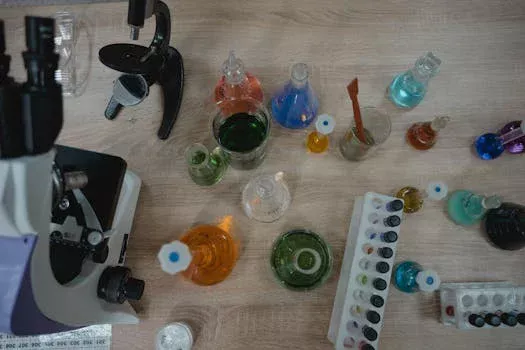
Polymer charge after coagulation follows particle charge, while lime dosing raises pH and precipitates hardness or metals before polymer feed bridges those solids into stronger flocs. Wrong polymer choice after coagulation wastes chemical and slows dewatering. Start with wastewater data before you lock chemistry. Plants that raise pH with alkali before the flocculant should read lime dosing process in water treatment explained as a separate equipment problem.
- Wastewater Characteristics: Measure zeta potential, pH (often 4–10), and particle size so charge and colloid load guide the first polymer pick.
- Cationic Polymers: Positive charge suits organic and biological solids in municipal, food, and pulp and paper streams. Dose is commonly 1–10 mg/L.
- Anionic Polymers: Negative charge suits solids after metal-salt coagulation (ferric chloride, alum), mining hydroxides, and many inorganic industrial loads. Dose is often 0.5–5 mg/L.
- Non-Ionic Polymers: Neutral bridging helps when charge swings or pH drifts, including some paper and textile cases. Dose is often 2–15 mg/L.
- Jar Testing Protocol: Adjust sample pH (for example 6–8), add polymer, mix 100 RPM for 1 minute, flocculate 30 RPM for 5 minutes, settle 10 minutes, then read residual TSS or turbidity.
- Cost Comparison: As of 2025 market data, cationic grades are about $3–$8/kg, anionic $2–$6/kg, and non-ionic $4–$10/kg, with bulk discounts common.
| Polymer Type | Charge | Typical Applications | Dosage Range (mg/L) | Approx. Cost (2025, $/kg) |
|---|---|---|---|---|
| Cationic | Positive | Organic matter, biological solids, food processing, municipal wastewater | 1–10 | $3–$8 |
| Anionic | Negative | Metal hydroxides, inorganic solids, mining, post-coagulation | 0.5–5 | $2–$6 |
| Non-Ionic | Neutral | Variable charge, paper mills, textiles, specialized industrial | 2–15 | $4–$10 |
According to a 2021 composite-polymer dosing study in IOP Conference Series, the optimum composite polymer dosage was 2.5 mg/L at an optimum pH 7. The jar test achieved 84.9%, 97%, and 92.4% removal of COD, turbidity, and TSS respectively. Treat 2.5 mg/L as one composite point inside the 0.5–10 mg/L jar-test band. It is not a permit limit, and it does not replace a site jar test when pH sits outside 6–8.
Seven Practical Ways to Raise Flocculation Efficiency
Flocculation changes can cut polymer use 15–25% while holding effluent quality and cake dryness. Most gains come from pH control, mixing energy, staged feed, and live turbidity feedback. Most plants we size for gain more from holding pH near 6–8 than from switching polymer brand.
- 1. Pre-Treat Wastewater: Hold influent near pH 6–8 and screen out large solids so polymer acts on colloids, not debris.
- 2. Optimize Mixing Energy: Keep rapid-mix G-values near 700–1000 s⁻¹ (per EPA 2023 guidelines), then drop to 20–70 s⁻¹ for gentle floc growth.
- 3. Gradual Dosing: Split addition into 2–3 points to build stronger flocs and limit local overfeed.
- 4. Monitor Turbidity: Inline clarified-stream turbidity control can cut polymer use 15–25% versus timed or flow-only feed.
- 5. Temperature Control: Keep solution near 15–25°C so viscosity and activity stay in range.
- 6. Regular Calibration: Monthly pump checks within ±1% flow tolerance prevent silent underfeed or overfeed.
- 7. Sludge Recirculation: Returning 10–20% thickened sludge can seed denser flocs and improve dewatering.
Operators comparing unit layouts can also review our detailed guide to flocculant dosing optimization for adjacent flocculant skid choices.
Common Failures and Field Fixes
Polymer feed failures usually trace to wrong charge, bad mixing, pump wear, or preparation faults. Fast diagnosis protects compliance and cloth life on the press. Most cloth-blinding calls we see start as excess feed, not as a defective cloth.
- Problem: Poor Floc Formation – Cloudy effluent or weak cake often means wrong polymer, G-value too low or too high, or off-spec pH. Re-run jar tests, retarget 700–1000 s⁻¹, and hold pH near 6–8.
- Problem: Polymer Overdosing – Viscous mixed liquor, cloth blinding, or large fragile flocs point to excess feed. If you see polymer dose too high in water, cut dose 10–20% and recalibrate the pump while watching TSS and cake release.
- Problem: Pump Clogging – Fish-eyes, debris, or line gel stop flow. Improve wetting and aging, add a 100-micron strainer, and flush lines weekly.
- Problem: Inconsistent Dosing – Worn tubing or diaphragms, air in the suction line, or bad flow sensors cause swingy floc quality. Calibrate monthly, replace wear parts, and purge air.
- Problem: High Sludge Volume – Weak or oversized flocs compact poorly. Retune mixing for denser flocs and re-test polymer grade for the dewatering machine.
- Problem: Foaming – High shear, excess polymer, or surfactants create foam. Lower G-value if needed, confirm dose, and dose antifoam at 0.1–0.5 mg/L only when surfactants are confirmed.
Day-to-day tank make-down and housekeeping steps are also covered in the boss solid solutions liquid polymer dosing tank operations manual style checklist used on many industrial skids.
Who This Skid Fits and the Next Step
Plant engineers, operators, and procurement teams use this guide when sizing polymer preparation and metering skids for industrial or municipal wastewater. Teams seeking only potable-water softening chemistry, or pure lime-slaker design without flocculant feed, should look elsewhere. Share flow, TSS, and the current polymer grade when you request a matched polymer dosing skid quote.
Most plants we size for send one week of flow and TSS, plus the polymer name and the last jar-test dose, before anyone picks a 50 L or 2000 L tank. That packet is enough to choose peristaltic or diaphragm duty and to test whether the 1.7 years example still holds at the site polymer price.
Frequently Asked Questions
What is the typical lifespan of these systems?
Major stainless tanks and frames often last 10–15 years, while pumps, sensors, and electronics commonly need replacement in 5–8 years. Annual maintenance and timely wear-part changes can extend overall life 20–30%. Most plants we size for keep the tank through two pump rebuilds, and they still budget the 5–8 year window for tubing, diaphragms, and probes.
How much does an automated polymer feed skid cost?
Manual or semi-automated packages often cost $5,000–$20,000. Fully automated industrial PLC systems typically cost $25,000–$100,000, driven by flow from 0.1–500 m³/h, tank size, and integration scope. The spread is mostly sensors, enclosure rating, and how far the PLC must reach the plant network. A pilot at the low end of 0.1–500 L/h should not be priced like a 2000 L tank with remote trim.
Can I use the same polymer for all wastewater types?
No. Charge, pH, and solids type change the winning grade, so one drum rarely covers every stream. Cationic grades are commonly dosed at 1–10 mg/L on organic solids, anionic at 0.5–5 mg/L after metal-salt coagulation, and non-ionic at 2–15 mg/L when charge swings. Jar testing still sets the grade and the working dose before the pump curve is locked.
How do I calculate the correct polymer dosage?
Dosage (mg/L) = (Polymer Flow Rate (L/h) / Wastewater Flow Rate (m³/h)) × Polymer Concentration (%). Example: 10 L/h of 0.2% (2000 mg/L) solution into 100 m³/h wastewater equals 2 mg/L. Most plants we size for start from that jar-test number and trim with turbidity instead of a fixed stroke. Recalculate whenever the wastewater flow or the solution strength changes.
What are the signs of polymer overdosing?
High mixed-liquor viscosity, filter-cloth blinding, excess foam, and large fragile flocs are common warnings of too much polymer. Reduce the dose 10–20% and recheck effluent TSS plus cake release. If foam is from confirmed surfactants rather than polymer, antifoam at 0.1–0.5 mg/L is the narrow fix, not a higher polymer stroke. Cut feed before you change the polymer grade.