What a Predictive Maintenance System for Sewage Treatment Actually Does
A predictive maintenance system for sewage treatment continuously ingests sensor data from critical rotating equipment, membrane trains and chemical dosing skids, runs anomaly detection and remaining-useful-life (RUL) estimation against a time-series historian, and auto-generates work orders 2–6 weeks before failure. The engineering definition that anchors this discipline is provided by the MathWorks Predictive Maintenance Toolbox documentation (2026): the software "lets you manage sensor data, design condition indicators, and estimate the remaining useful life (RUL) of a machine" using "statistical, spectral, and time-series analysis." That framing separates PdM from calendar-based preventive maintenance, which schedules work on elapsed time, and from reactive maintenance, which runs after the asset has already failed.
For a 5,000–500,000 PE plant, the asset classes that justify instrumenting first are the ones with the highest cost-per-failure-hour: aeration blowers (typically 30–60% of plant electrical load, per typical WWTP energy audits), MBR membrane modules, UV lamp arrays, chemical dosing pumps, rotary bar screens, and decanter centrifuges or sludge dewatering presses. MBR membrane bioreactor systems and other rotating equipment are the dominant reliability risk because they run continuously and their failure modes — fouling, bearing spall, sleeve scaling — are detectable in the 2–8 week precursor window if the right sensors are installed.
This article is a vendor-agnostic engineering guide for selecting, sizing and defending a PdM retrofit. It assumes the reader already runs SCADA and a digital twin engineering guide for WWTPs is on the roadmap, and that the immediate question is what to instrument, what model to run, and how to justify the spend to a finance director.
The Five-Layer Architecture: From Sensor to Work Order
Every PdM stack in a sewage plant collapses to five layers, and each layer has non-negotiable engineering constraints that differ from a generic factory deployment. Layer 1 is the field sensor set: IEPE accelerometers with 1–10 kHz bandwidth on bearing housings, motor current signature analysis (MCSA) clamps on the power feed, PT100 RTDs on bearing housings and windings, 4–20 mA pressure transmitters with ±0.5% FS accuracy for transmembrane pressure (TMP), free chlorine probes, and turbidity sensors. Wet-well and headworks locations should be specified to IP68 to survive hosing and submergence; the same applies to bar screen motor enclosures exposed to splash.
Layer 2 is the edge gateway, which does protocol translation (Modbus RTU/TCP, PROFINET, EtherNet/IP, IO-Link Wireless) and publishes to MQTT. Edge buffering matters more in WWTPs than in most factories: rural plants commonly have 10–60 minutes of WAN outage per day, and the gateway must store-and-forward at full vibration sample rates to avoid blind spots. Layer 3 is the time-series historian. OSIsoft PI remains the dominant choice for brownfield sites that already run it; InfluxDB or open-source TimescaleDB are credible at 1 Hz minimum sampling and sub-second where vibration is captured. Layer 4 is the ML inference engine, typically containerised under Docker or Kubernetes with a model registry, A/B testing, and drift monitoring. The MicaelSoares7/predictive-maintenance-api GitHub repository (updated Feb 19 2025) describes the canonical pattern of "integrating IoT sensors and ERP systems" so the API can "detect anomalies and predict failures before they happen" — the same architecture applies to a 50,000 m³/day plant with OSIsoft PI feeding an MLflow model registry. Layer 5 is the CMMS/EAM bridge — SAP PM, IBM Maximo, or open-source iTop — over REST, which turns a model score into a work order with RUL, recommended parts, and a job plan. This kind of DCS system selection for wastewater plants integration is where most projects stall, so it should be specified up front, not bolted on at month 11.
Sensor Bill of Materials by WWTP Asset
Below is a starting BOM a plant engineer can hand to a vendor RFQ. Unit costs in the 2026 market are in the $300–$1,200 range per sensor point for industrial-grade instruments; the wider band for blower and MBR packages reflects whether the accelerometers are top-tier IEPE brands or commodity MEMS (industry-typical range, verify with vendor RFQ). IP68 is mandatory for any sensor within splash or wash-down range of the asset.
| Asset class | Sensors (per unit) | Signal / sampling | IP rating | 2026 unit cost (USD) |
|---|---|---|---|---|
| Aeration blower (75 kW turbo) | 2× IEPE accelerometer, 1× MCSA clamp, 1× PT100 RTD | Vibration 1–10 kHz; current 1–4 kHz; temperature 1 Hz | IP67 / IP68 | $1,800–$3,800 |
| MBR membrane module (PVDF) | 1× TMP transmitter (±0.5% FS), 1× aeration flow, 1× temperature | Pressure 1 Hz; flow 1 Hz; temperature 1 Hz | IP68 wet-end | $1,200–$2,600 |
| UV disinfection bank | 1× 254 nm intensity, 1× lamp hours counter, 1× ballast RTD, 1× ΔP for sleeve fouling | Optical 0.1 Hz; digital counter; temperature 1 Hz; pressure 1 Hz | IP65 | $1,400–$2,800 |
| Chemical dosing pump | 1× flow verification, 1× diaphragm pressure, 1× day-tank level | Pulse/4–20 mA; pressure 1 Hz; level 0.1 Hz | IP65 | $900–$1,900 |
| Rotary bar screen | 1× motor current, overload trip counter, rake-torque proxy (current-derived) | Current 1 Hz; digital event | IP65 | $600–$1,400 |
| Plate and frame filter press | 1× hydraulic pressure, 1× feed pump current, cycle-time counter | Pressure 1 Hz; current 1 Hz; digital event | IP65 | $700–$1,600 |
For plants scoping a full retrofit, integrated packages such as MBR membrane bioreactor systems, DF series flat sheet MBR modules, GX series rotary bar screens, plate and frame filter press for sludge dewatering, and automatic chemical dosing systems are common asset-class anchors for the PdM stack because they ship with the instrumentation taps needed to mount the sensors above.
Choosing the Right ML Model: LSTM vs Random Forest vs Survival Analysis
Model choice on a WWTP PdM project should be driven by data volume, failure-tag maturity, and interpretability need — not by vendor accuracy claims on benchmark datasets. The five model families that matter, and their fit, are summarised below.
| Model family | Best fit on WWTP PdM | Training data need | Interpretability | Compute footprint |
|---|---|---|---|---|
| LSTM / Temporal CNN | High-frequency vibration & current on critical assets with 6+ months of failure-tagged history | 10,000+ labelled windows | Low (SHAP on attributions) | GPU recommended |
| Random Forest / XGBoost on engineered features (RMS, kurtosis, spectral kurtosis) | Default choice for ~70% of WWTP deployments; works with 50–500 labelled events | 50–500 failures | High (SHAP values) | CPU only |
| Survival analysis (Cox PH, Weibull AFT) | Censored "time-to-next-overhaul" data; aligns with RUL toolboxes such as MathWorks Predictive Maintenance Toolbox (2026) | 100–1,000 records with censoring | Medium | CPU only |
| Isolation Forest / autoencoder | Untagged assets where failures are rare; trades false-positive rate for coverage | Unsupervised | Low–medium | CPU only |
Decision rule: instrument the asset, baseline for 60–90 days, then start with feature-engineered tree models plus statistical control limits (CUSUM, EWMA). Escalate to LSTM or survival analysis only on the top three critical assets where the data volume justifies the data-science cost. This sequencing mirrors the staged approach in an AI process control guide for industrial wastewater and avoids the common failure of a deep-learning pilot that has no labelled failures to learn from.
Failure-Mode Library: The Real Source of PdM Value

The model accounts for roughly 20% of PdM value; the curated failure-mode library accounts for the other 80%. Every signature in the library needs a precursor tag list, a threshold, a lead-time window, a recommended action, a parts kit, and a safety class. A few examples that drive the bulk of the savings on a typical plant:
- Blower bearing outer-race spall — 4–8 week precursor in high-frequency vibration kurtosis on the drive-end accelerometer; lead action is grease analysis and alignment check, then a replacement bearing kit sized to the blower model.
- MBR membrane irreversible fouling — 5–14 day precursor in TMP rate-of-change; lead action is an in-situ chemical clean, escalating to replacement evaluation if the recovery is below threshold. This signature ties directly to an $80K–$200K membrane capex event (verify with vendor pricing) and is the single highest-ROI failure mode in MBR plants.
- UV lamp end-of-life — 2–4 week precursor in 254 nm intensity drop combined with ballast temperature rise; replace lamp and quartz sleeve as a kit on a planned shutdown.
Building this library is a documentation project as much as a data-science project. The spare parts and consumables OPEX guide framing is useful here because every signature has to resolve to a kit that actually sits on a shelf.
Building the Business Case: ROI and Payback Worksheet
There are three savings levers in a PdM business case, and a defensible number set should quantify all three. The first is avoided unplanned downtime; the second is extended maintenance intervals (calendar-based to condition-based, typically 1.3–1.8× extension on rotating equipment); the third is reduced spare-parts inventory via just-in-time replenishment (typically 15–25% working-capital release on rotating-equipment SKUs). Downtime cost at a medium-sized WWTP sits in the $10K–$50K per hour of unplanned outage range, driven by permit excursion risk and bypass pumping — this is an industry-typical band, validate with the plant's own incident log (HydropureWater field data, 2026).
For a 10,000 m³/day retrofit, capex typically lands in the $250K–$900K band covering sensors, edge, historian, ML platform and integration; opex is $40K–$120K/year for licensing and data engineering (verify with vendor RFQ). The payback formula is (annual downtime-cost avoided + labor savings + spare-parts reduction) ÷ (annual opex + amortized capex), which on most retrofits lands at 18–36 months. PdM is no longer an experimental line item: mainstream business press is documenting manufacturer PdM investment as a 2026 baseline capability (Footwear News, 22 June 2026), and water utilities are now in the same procurement wave.
| Line item | Conservative | Typical | Notes |
|---|---|---|---|
| Capex (10,000 m³/d retrofit) | $250K | $900K | Sensors, edge, historian, ML, integration |
| Opex (annual) | $40K | $120K | Licensing + data engineering |
| Downtime cost (per hour) | $10K | $50K | Permit excursion + bypass pumping |
| Maintenance interval extension | 1.3× | 1.8× | Calendar → condition-based |
| Spare-parts working-capital release | 15% | 25% | Just-in-time replenishment |
| Payback window | 36 mo | 18 mo | Net of amortized capex |
The numbers above are intentionally bracketed; the engineering work is to replace each cell with a plant-specific value drawn from the SCADA historian, the CMMS, and the procurement system. The companion TCO breakdown for a wastewater treatment plant lays out how those figures tie into the wider O&M budget.
Phased Rollout: 90 / 180 / 365-Day Implementation Plan
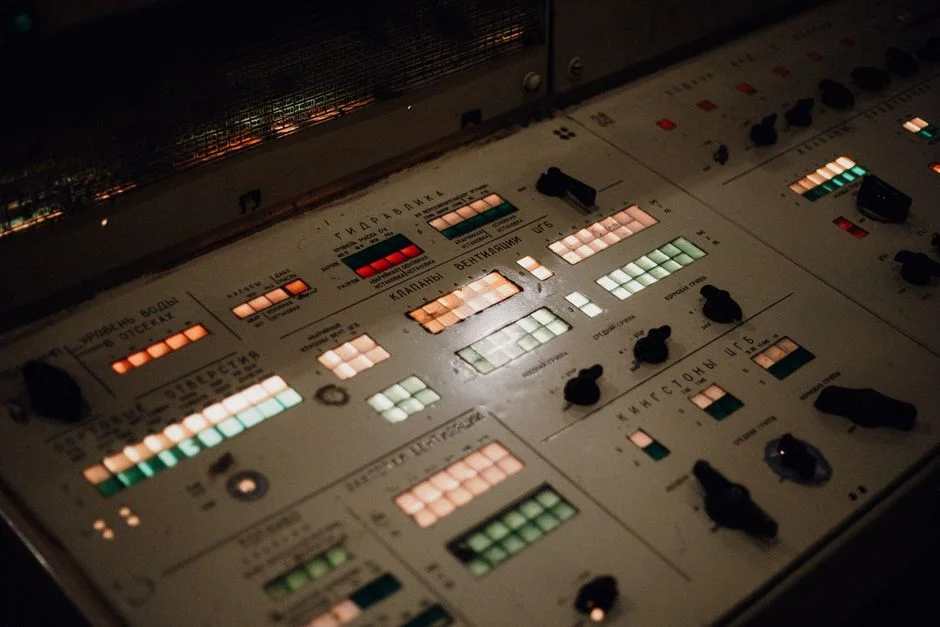
A small O&M team can execute a credible PdM rollout in three phases totalling one year.
- Days 0–90 — Pilot. Instrument two critical assets (one aeration blower, one MBR train), baseline for 60 days, train a feature-engineered tree model with CUSUM/EWMA control limits, and deliver the first three automated work orders against the failure-mode library.
- Days 91–180 — Expand. Add chemical dosing and UV bank instrumentation, grow the failure-mode library to 30+ signatures, integrate with the CMMS via REST, and stand up historian dashboards for the operations team.
- Days 181–365 — Scale. Roll out across all blowers and MBR trains, introduce LSTM or survival analysis for the top critical assets, and lock in a quarterly model retraining cadence.
Common failure modes of PdM programs themselves include sensor calibration drift, model staleness as operating points shift, and alert fatigue from low-precision models. Schedule a quarterly model performance review and tie it to a written drift report — this is the same discipline applied to pH and ORP controller tuning on a wastewater plant, and it is what separates a working PdM stack from a dashboard nobody trusts.
Frequently Asked Questions
What is a predictive maintenance system for sewage treatment in one sentence, and what are the three minimum sensors per asset?
A PdM stack continuously ingests sensor data, runs time-series models, and auto-generates work orders 2–6 weeks before failure; the minimum sensor set per critical asset is one vibration point, one process variable (pressure, flow or TMP), and one temperature point.
What payback can a 10,000 m³/day plant realistically expect from a 2026 retrofit?
18–36 months on a $250K–$900K capex, assuming the three savings levers (avoided downtime, extended intervals, spare-parts release) are all quantified and the downtime-cost band of $10K–$50K/hour is calibrated to the plant's incident log.
Are open-source stacks (InfluxDB + Python + MLflow) production-grade for WWTPs?
Yes, for plants with internal data-engineering capacity; OSIsoft PI and enterprise CMMS suites still win on long-term support and audit trails, which matters under permit-driven compliance regimes.
Which MBR TMP threshold should trigger a clean-in-place recommendation?
A sustained rise of 10–20% above the clean-membrane baseline at constant flux, or a TMP rate-of-change exceeding the rolling 7-day average by 1.5–2×, is the conventional trigger window; finalise the threshold against vendor recovery data for the specific module.
How do I justify the project when the plant has no PdM budget line?
Reframe it as an OPEX reduction programme (avoided downtime, extended PM intervals, spare-parts working-capital release) rather than a capex line; the 18–36 month payback window will usually beat the cost of the next unplanned excursion.