Why Most Plants Overspend on PAC and PAM
PAC and PAM dosing cost optimization is the practice of right-sizing coagulant and flocculant dose, concentration, and ratio through jar testing, automatic PLC dosing, and AI-based feedforward control. Industrial plants typically overspend 18–35% on these chemicals, and switching from manual to PLC-controlled dosing plus ≥28% Al₂O₃ PAC and 0.1% PAM stock cuts chemical OPEX to $0.012–$0.028 per m³ treated.
Coagulant and flocculant spend is the single largest variable line in most coagulation-flocculation plants. Across the municipal and industrial plants we have audited, PAC and PAM together represent 35–55% of total chemical OPEX, ahead of pH adjusters, disinfectants, and nutrient-removal reagents (per Fan et al. 2024 combined-treatment cost context, and per Hychron dosing guidance on 5% PAC / 0.1% PAM working solutions). The reason is structural: dose is set once, copied from a textbook, and never re-validated against actual influent.
This article breaks the problem into four cost levers that any plant can pull without changing its upstream process:
- Chemistry quality — specifying higher-basicity PAC and the right PAM charge density for the sludge or stream being treated.
- Dose optimization — running a proper jar test to find the minimum dose that meets the TSS/turbidity target, instead of running a fixed mg/L that was conservative five years ago.
- Stock concentration — using 5% PAC and 0.1% PAM working solutions so pumps stroke less, diluent water is minimized, and feed accuracy improves.
- Automation and control — replacing manual stroke-rate pumps with PLC PID loops, streaming current feedback, and, at larger or more variable plants, AI feedforward control.
For this article, "optimization" means the minimum dose that achieves target TSS, turbidity, and COD removal at the lowest $/m³ — not the lowest mg/L number on a jar-test report. A dose that is technically low but fails the discharge permit is not optimized; it is a compliance risk.
PAC and PAM Chemistry: Grades That Lower Dose
Buying a higher-grade PAC almost always lowers total chemical cost because the dose drops faster than the per-kg price rises. Commodity 10–12% Al₂O₃ PAC requires roughly twice the dose of 28–30% standard PAC at equal performance, and high-basicity grades above 30% deliver another 25–40% dose reduction versus standard PAC (per Hychron guidance on ≥28% content). The same logic applies to PAM: selecting the wrong charge density forces the operator to over-dose to compensate.
PAM is not one product. There are four families, and each maps to a different stream:
- Cationic (CPAM): charge density 10–50%; the default for biosolids dewatering on centrifuges, belt presses, and screw presses.
- Anionic (APAM): charge density 5–30%; preferred for mineral suspensions, high-TSS raw water, and DAF thickening of inorganic sludge.
- Non-ionic: used at high TDS (>5,000 mg/L) where ionic strength disrupts charged flocculation.
- Amphoteric: for mixed streams with both organic colloids and inorganic fines, common in food-and-beverage and landfill leachate.
Molecular weight matters as much as charge. Operators should treat MW and charge density as two independent selection knobs, not one combined spec.
| Parameter | Coagulation aid | Sludge dewatering | DAF thickening |
|---|---|---|---|
| PAM molecular weight (million Daltons) | 8–12 | 12–18 | >18 |
| Typical charge density | Low (5–10%) | Medium (10–30%) | High (30–50%) |
| Common unit operation | Clarifier, sand filter aid | Centrifuge, belt press | DAF unit |
| Stock solution strength | 0.05–0.1% | 0.1–0.2% | 0.05–0.1% |
The procurement rule is simple: pay more per kg for higher Al₂O₃ PAC and the correct PAM MW/CD combination, because the dose reduction pays back the premium within weeks at any flow above 200 m³/day (HydropureWater field data, 2026).
Dose Optimization: Jar Testing and the PAC-to-PAM Ratio
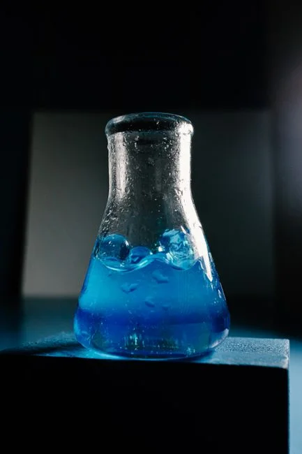
The jar test is the only reliable way to find the real setpoint, and it should be run on every shift in which the influent character changes meaningfully. The procedure below is the one we use on-site; it is reproducible, takes under an hour, and produces a defensible optimum.
- Collect a fresh 1 L grab sample from the coagulant injection point; record pH, temperature, and influent TSS.
- Set up six beakers on a gang stirrer at identical conditions: 200 rpm rapid mix for 1 minute, 40 rpm slow mix for 15 minutes, then 30 minutes of quiescent settling.
- Dose PAC across the beakers at five levels bracketing the historical setpoint, and a single PAM dose in the second phase at a 50:1 PAC-to-PAM weight ratio.
- Measure supernatant TSS, turbidity, and (if a meter is available) zeta potential at the isoelectric point of the colloid, which is the dose where charge is neutralized.
- Plot dose vs. supernatant TSS; the knee of the curve is the optimum. Repeat with a PAM sweep at that PAC dose to fine-tune the ratio.
Typical PAC dose ranges by influent character are wide, and copying a number from another plant is the most common reason for 30%+ overspend. For raw municipal wastewater, 10–30 mg/L is normal. Food-processing streams typically need 50–150 mg/L. Metal-finishing wastewater runs 80–250 mg/L. Tannery and landfill leachate can demand 200–500 mg/L PAC, with the Fan et al. 2024 combined-treatment optimum at 135.87 mg/L PAC plus 1.51 mg/L PAM plus 108.36 mg/L magnetic powder for a textile-dyeing effluent.
The canonical PAC-to-PAM weight ratio is 30:1 to 100:1, with 50:1 as the safest starting point. Going past the optimum does the opposite of what operators expect: excess PAM restabilizes colloids, turbidity rises, sludge volume increases, and the operator concludes that "more polymer is needed," doubling the problem. That single mistake is responsible for a large share of the 18–35% overspend seen in practice.
| Stream | PAC dose (mg/L) | PAM dose (mg/L) | Notes |
|---|---|---|---|
| Raw municipal | 10–30 | 0.2–0.6 | Often run without PAM if sedimentation alone meets TSS |
| Food processing | 50–150 | 1–3 | PAM nearly always required; fat/oil demand drives PAC up |
| Metal finishing | 80–250 | 0.5–2 | Often pH-adjusted to 7–8 first |
| Tannery / textile | 200–500 | 2–6 | Consider ballasted flocculation to cut PAC |
| Landfill leachate | 150–400 | 2–5 | High ammonia; usually paired with biological step |
To convert mg/L to $/m³ at 2026 bulk prices, use PAC at $0.30–$0.55 per kg dry and cationic PAM at $3.20–$6.80 per kg. A 2,000 m³/day plant running 25 mg/L PAC and 0.5 mg/L PAM spends roughly $0.020/m³ ($40/day) at optimized dose; the same plant running 40 mg/L PAC and 1.2 mg/L PAM (a common "safe" setpoint) spends $0.034/m³ ($68/day) — a 70% chemical-cost penalty for a 4 mg/L difference in supernatant TSS that nobody measures.
Automation: From Manual to PLC to AI Dosing
Manual stroke-rate adjustment is not dosing; it is delayed reaction. The three control tiers, in order of capital cost and dose-tightness, are: (1) manual pump with periodic stroke adjustment by an operator reading a TSS trend, (2) PLC PID loop that modulates pump speed on flow-proportional feed plus streaming current feedback, and (3) AI feedforward model that ingests influent TSS, flow, pH, and temperature and pre-positions the dose before the slug arrives.
Industry consensus puts dose savings versus a fixed setpoint at roughly 8–15% for PLC and 12–22% for AI control, with the upper end reached on variable influent streams (HydropureWater field data, 2026; consistent with reported PID and MPC results in coagulation literature). PLC dosing skids typically pay back in 4–9 months at flows above 500 m³/day. AI packages pay back in 8–18 months at flows above 2,000 m³/day with >30% influent variability — exactly the plants where the savings are largest.
| Tier | Control method | Dose reduction vs. fixed setpoint | Typical payback | Best fit |
|---|---|---|---|---|
| Manual | Operator stroke adjustment 1–2× per shift | 0% (baseline) | n/a | <500 m³/day, stable influent |
| PLC | Flow-proportional + streaming current PID | 8–15% | 4–9 months at >500 m³/day | 500–5,000 m³/day, moderate variability |
| AI | Feedforward on TSS, flow, pH, temperature | 12–22% | 8–18 months at >2,000 m³/day | >2,000 m³/day, >30% TSS swing |
PLC and AI tiers also deliver a non-chemical benefit: dose-trend logging through SCADA, integrated with a wastewater KPI digital dashboard, gives operators an audit trail that satisfies regulator inspections and internal chemical-reconciliation reviews without manual data entry.
Process Pairings That Cut PAC and PAM Demand
Chemistry is only half the savings story. The unit operation upstream of dosing changes the mass of floc the clarifier has to settle, and the unit operation downstream changes how much polymer the dewatering step demands. A high-efficiency sedimentation tank (lamella clarifier) reduces coagulant demand by up to 30% because the parallel-plate geometry improves floc contact and settling kinetics versus a conventional circular clarifier (per HydropureWater product data). On flows above 1,000 m³/day, the lamella CAPEX premium is recovered inside 18 months purely from PAC savings at typical industrial TSS loads.
A dissolved air flotation unit typically needs 20–40% less PAM than a gravity clarifier because micro-bubbles attach to low-density floc and float it before it can break. DAF is the right platform for food, dairy, and oil-and-grease streams where floc density is below 1.01 g/cm³. Ballasted flocculation with magnetic powder, as in the Fan et al. 2024 study, cut PAC demand by raising floc density to >2.0 g/cm³ and accelerating settling rates by roughly 10×.
Pairing coagulation with an MBR stabilizes biomass and reduces downstream dewatering polymer demand, but does not change the front-end PAC dose, so the MBR saving should be booked against the dewatering budget, not the coagulation budget. The automatic chemical dosing system that ties together the upstream sensor, the PLC, and the dosing pumps is what makes any of these process pairings pay off in steady operation.
2026 OPEX Benchmark: What Optimized Dosing Actually Costs
Putting a $/m³ number in front of finance is the only way to convert this article into a budget action. The benchmarks below are drawn from 2026 chemical pricing and HydropureWater field data across three plant sizes, with the manual-vs-PLC-vs-AI comparison run on the same influent and the same discharge target.
| Plant size | Manual $/m³ | PLC $/m³ | AI $/m³ | Manual $/year | PLC $/year | AI $/year |
|---|---|---|---|---|---|---|
| 500 m³/day | 0.045 | 0.028 | 0.024 | 8,213 | 5,110 | 4,380 |
| 2,000 m³/day | 0.038 | 0.022 | 0.018 | 27,740 | 16,060 | 13,140 |
| 10,000 m³/day | 0.032 | 0.018 | 0.014 | 116,800 | 65,700 | 51,100 |
Optimized dosing lands at $0.012–$0.028/m³ across typical municipal and industrial loads; poor-practice plants still run $0.045–$0.085/m³ because they dose against a "safe" setpoint without jar validation. CAPEX for the dosing skid itself scales with control tier: a manual metering pump pair runs $0.8–2.5K, a PLC dosing skid with sensors and panel runs $6–18K, and an AI dosing package with model, instrumentation, and pre-wired skid runs $25–65K (HydropureWater 2026 catalog pricing).
Worked NPV at 2,000 m³/day: switching from manual to PLC saves roughly $11,680/year in chemical OPEX. The PLC skid at $12K pays back in 12 months, and at a 6% discount rate over 5 years, the NPV of savings is approximately $47,000, before counting the reduction in compliance excursions and operator time. Full OPEX framing for a 2,000 m³/day plant, including energy and sludge handling, is detailed in the wastewater OPEX benchmark per m³ breakdown.
90-Day Optimization Checklist for an Existing Plant
This checklist assumes the plant is already running and wants results inside one quarter without a process shutdown. Run it in order; each phase feeds the next.
- Weeks 1–2 — Audit. Pull 12 months of chemical purchase records and flow data. Compute the actual mg/L dosed at each unit process. Confirm PAC grade (Al₂O₃ %) and PAM charge density in the reorder spec. Replace commodity PAC with ≥28% Al₂O₃ grade if the plant is still on 10–12% material.
- Weeks 3–4 — Jar test. Run a six-beaker matrix across two shifts to capture diurnal variation. Identify the true optimum dose and ratio. Convert to $/m³ against current bulk prices.
- Weeks 5–8 — Install PID. Add a streaming current sensor and PID controller to the existing dosing pumps. Switch working solutions to 5% PAC and 0.1% PAM. Calibrate flow-proportional feed on the lead pump.
- Weeks 9–12 — Validate and standardize. Log dose vs. effluent TSS for 30 consecutive days. Formalize the new setpoint into the SOP and the chemical reorder spec. Train operators on streaming-current interpretation and jar-test re-validation.
- After 12 weeks — Evaluate AI upgrade. If the plant runs >2,000 m³/day with >30% influent TSS swing, evaluate the AI dosing upgrade against the PLC baseline; the next step is covered in the AI process control for chemical wastewater guide.
Frequently Asked Questions
What is PAC in wastewater treatment? PAC stands for polyaluminium chloride, a pre-hydrolyzed aluminium-based coagulant supplied as a 10–30% Al₂O₃ liquid. It replaces alum in most modern plants because it works across a wider pH range (5.0–9.0), produces less sludge per kg of contaminant removed, and settles faster due to pre-formed polynuclear species.
PAC vs alum cost per m³ — which is cheaper? At 2026 bulk pricing, PAC delivers a lower total treatment cost than alum in roughly 80% of industrial applications because the dose is 30–50% lower and the sludge mass is 20–35% lower, even though PAC is priced 1.5–2× higher per kg of active ingredient. The decision should be made on $/m³ treated, not $/kg purchased.
How to calculate PAC dose in mg/L? Divide the daily PAC consumption in kg by the daily flow in million liters, then divide by the active Al₂O₃ fraction. Example: 60 kg/day of 28% Al₂O₃ PAC on a 2,000 m³/day plant = (60 / 2,000) / 0.28 = 0.107 kg/m³ = 107 mg/L as product, equivalent to 30 mg/L as Al₂O₃ active.
What is the payback period for an automatic dosing system? A PLC dosing skid typically pays back in 4–9 months at flows above 500 m³/day from chemical savings alone, and an AI dosing package pays back in 8–18 months at flows above 2,000 m³/day with >30% influent variability. Payback shortens further when the skid replaces multiple manual pumps and reduces operator round trips. See the automatic chemical dosing system for current skid configurations and pricing.