What a Remote Monitoring System for Wastewater Treatment Actually Does
A remote monitoring system for wastewater treatment is the continuous, sensor-based acquisition of process and equipment data — pH, dissolved oxygen, ORP, TSS, NH3-N, flow, level — transmitted from the plant to a central SCADA server or cloud platform where it becomes trends, alarms, and audit records (Racoman, 2024-04). The function is telemetry and visibility, not closed-loop control: a remote monitoring system tells the operator that dissolved oxygen in basin 2 dropped to 1.2 mg/L; a control system would then command the blower VFD to ramp up. Most industrial plants start with monitor-only and migrate to control after 6–12 months of stable data, because control logic on a noisy signal is the most common way to burn out an aeration blower in week one.
The economic case rests on two value streams. The first is labor: a typical 1,000 m³/day plant running 16 daily manual checks (HydropureWater field data, 2025) can cut routine site-visit hours by 40–60% once reliable online sensors replace hand-held probes. The second is risk: earlier detection of excursions before discharge-limits are breached. As Digi International notes, wireless monitoring delivers water level, flowage, and performance data so plant managers can make quicker, more informed decisions — and that visibility is what converts a permit violation from a six-figure event into a logged alarm that an operator clears before sunrise. On the chemical side of the plant, the same architecture drives a PLC-controlled chemical dosing skid, where flow-paced injection replaces timer-based dosing and cuts coagulant consumption 8–15%.
System Architecture: From Sensor in the Aeration Tank to the Operator's Browser
An industrial deployment breaks cleanly into four functional layers, and the layers — not the brand names — are what a controls engineer should specify first.
Layer 1 — Field sensors. The measurement layer is dominated by pH (glass-body, 0–14), dissolved oxygen (optical or galvanic membrane), ORP, TSS (optical or ultrasonic), NH3-N (ion-selective electrode), conductivity, magnetic or ultrasonic flow, hydrostatic or radar level, ClO₂ residual (amperometric), and turbidity. Most probes output 4–20 mA or Modbus RTU at 1–10 second sample intervals; high-end optical DO and TSS probes now publish on Modbus TCP at 1 Hz for closed-loop aeration control.
Layer 2 — RTU/PLC. Industrial controllers aggregate sensor signals, log locally to non-volatile memory (typically 32–256 MB), and buffer data through cellular or mesh outages. Modbus TCP, PROFINET, and EtherNet/IP are the three fieldbus choices that cover roughly 90% of greenfield installations in 2026; PROFINET dominates in European municipal work, EtherNet/IP in North American industrial, Modbus TCP everywhere else.
Layer 3 — Communication gateway. A cellular 4G/5G or LTE-M/NB-IoT modem, a LoRaWAN 8-channel gateway, a Wi-SUN mesh node, or a fiber backhaul connects the RTU to the outside world. Selection depends on site geography, endpoint count, and the IT/OT network boundary — see the technology comparison in the next section.
Layer 4 — SCADA/cloud platform. Dashboards, SMS/email alarming, historical trending on a 1-second to 1-year timebase, and optional AI/ML modules for aeration and chemical-dose optimization. On-premise SCADA (Ignition, FactoryTalk, WinCC) is preferred where data sovereignty or air-gap cybersecurity rules apply; SaaS platforms (AWS IoT, Azure Industrial IoT) win on multi-site rollouts. For plants ready to close the loop on aeration, the natural next read is our AI process control engineering guide.
Choosing the Communication Technology: Cellular vs LoRaWAN vs Wi-SUN
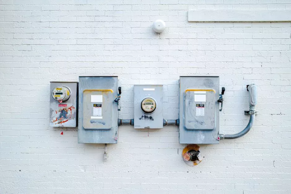
The wireless backhaul decision is driven by three numbers: how many endpoints, how far apart, and how much data per endpoint per minute. Get those wrong and the rest of the architecture inherits the mistake.
| Criterion | Cellular 4G/LTE-M/NB-IoT | LoRaWAN | Wi-SUN |
|---|---|---|---|
| Typical data rate | 0.1–10 Mbps | 0.3–50 kbps | 50–300 kbps |
| Range, line of sight | Cell-tower dependent (1–10 km typical) | 2–10 km | 1–5 km per hop, mesh-extended |
| Endpoint battery life | Powered or rechargeable; 1–5 yr on Li | 5–10 years on 2.4–8.5 Ah Li | Powered (mains or solar); 1–3 yr battery |
| Per-device monthly cost | $5–$25 (data plan) | $0–$3 (unlicensed spectrum) | $0 (unlicensed) + gateway OPEX |
| Best fit | Dispersed sites: lift stations, pumping stations, remote headworks | Dense on-site sensor mesh inside one plant | Multi-plant municipal AMI, >1,000 endpoints |
| Limitation | Carrier coverage gaps; recurring OPEX | Low payload — not for video or waveforms | Higher gateway capex; mesh tuning |
| Cybersecurity baseline | Private APN or IPSec VPN | LoRaWAN 1.1.x with AppKey per device | Wi-SUN FAN 1.1 with IEEE 802.15.4g security |
Decision rule: dispersed remote sites → cellular; on-site dense sensor mesh → LoRaWAN; multi-plant municipal AMI → Wi-SUN. Fiber or wired Ethernet remains preferred for the SCADA backbone inside the plant, where determinism and immunity to RF noise matter more than the cost of pulling cable.
Which Parameters to Monitor at Each Process Stage
The matrix below is the shortest path between "we have to monitor the plant" and a defensible I/O list. Match the parameter to the process failure mode it actually detects.
| Process stage | Primary parameters | Sensor type | Failure mode detected |
|---|---|---|---|
| Headworks / screening | Flow, level | Magnetic flowmeter; ultrasonic or radar level | Pump cavitation, ragging, overflow |
| Primary / equalization | pH, TSS | Glass-body pH; optical or ultrasonic TSS | Toxic slug load to aeration |
| Biological (A/O, SBR, MBR) | DO, ORP, temperature, NH3-N | Optical or galvanic DO; ISE NH3-N | Nitrification failure, energy waste |
| Disinfection | ClO₂ or Cl₂ residual, turbidity | Amperometric residual; turbidity | Discharge-limit breach, reuse failure |
| Effluent (final) | COD, TSS, pH, flow | UV absorption COD; optical TSS; pH; magmeter | Direct permit exceedance |
DO control on its own typically cuts aeration energy 15–25% in activated-sludge plants (HydropureWater field data, 2025), which is why the biological stage is the highest-leverage place to put a transmitter. For the screening step upstream, a rotary mechanical bar screen paired with a level transmitter prevents the ragging events that take a bar screen's downstream pump out. Disinfection needs a residual loop that is closed against flow, served by an on-site ClO₂ generator with online residual feedback. Plants on tight footprints or with reuse targets should consider an MBR membrane bioreactor system, which raises effluent quality and tightens the monitoring spec at the same time.
Sensor Selection, Calibration, and Maintenance Discipline
The most expensive sensor in the catalog is the one that drifts in the field and is never recalibrated. Body material must match the matrix: PVC for municipal, PVDF/PP or 316L stainless for chemical and high-TDS industrial streams, Hastelloy for hot chloride service above 60 °C. Optical DO and optical TSS probes need 2–4 cleanings per year and produce stable readings for 3–5 years; membrane DO probes need membrane replacement every 3–6 months and electrolyte refill on the same cadence. Build that labor into OPEX, not into the contingency line.
Online NH3-N ion-selective electrodes require buffer calibration monthly and probe replacement every 6–12 months in fouling service — gas-phase ISE units (no direct sample contact) extend that to 12–18 months but cost roughly 1.8× a wet-contact probe. Always specify auto-cleaning ultrasonic or mechanical wiper attachments on optical probes in FOG- or fiber-laden streams (food processing, pulp and paper, textile); without them, TSS optical probes lose correlation in 2–3 weeks. For oily streams, the right upstream measurement is covered in our online oil and grease monitoring sensor guide.
Cybersecurity, Standards, and Regulatory Mapping
Remote access is no longer optional — and neither is the conversation with the IT security team. Apply IEC 62443-3-3 zoning: the remote-monitoring VLAN sits in a separate security zone from corporate IT, with explicit conduits defined for each data flow. Cellular links terminate on a private APN or IPSec VPN, not on the public internet. PLC firmware and SCADA credentials rotate quarterly, and any remote-access session is brokered through a jump host with full session recording.
Mapping monitoring to the permit is the second half of the compliance picture. Under the EU Urban Wastewater Treatment Directive (91/271/EEC), typical discharge ceilings are BOD ≤30 mg/L, COD ≤125 mg/L, NH3-N ≤10 mg/L, TSS ≤30 mg/L; equivalent EPA NPDES and Chinese GB 18918-2002 limits are within the same order of magnitude. Continuous monitoring records are increasingly accepted in lieu of manual composite sampling for some parameters, which reduces lab OPEX by $8K–$25K per year at a mid-size plant (HydropureWater field data, 2025). Audit trail must log every setpoint change, alarm, and acknowledgement to satisfy ISO 14001 inspections and discharge-permit audits. For NH3-N specifically, see our online ammonia nitrogen analyzer engineering guide.
Cost Structure and 3-Year ROI for a Mid-Size Industrial Plant
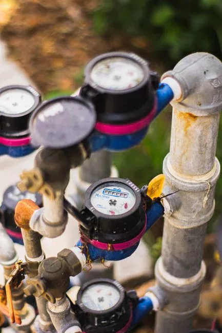
The business case has to survive procurement, finance, and the plant manager's "what does it save me" question. The numbers below are for a 500–2,000 m³/day industrial plant with 8–15 sensor channels.
| Line item | Year 1 | Year 2 | Year 3 | Notes |
|---|---|---|---|---|
| CAPEX — sensors + RTU + gateway + SCADA license | $40K–$120K | $0 | $0 | Scales with channel count and SCADA tier |
| Integration & commissioning | $20K–$60K | $0 | $0 | One-time engineering |
| OPEX — cellular data ($5–$25 × 12 × devices) | $0.7K–$4.5K | $0.7K–$4.5K | $0.7K–$4.5K | Per device per month |
| OPEX — sensor maintenance (5–10% of CAPEX) | $2K–$12K | $2K–$12K | $2K–$12K | Calibration, membranes, wipers |
| OPEX — SCADA SaaS or license support | $2.4K–$18K | $2.4K–$18K | $2.4K–$18K | $200–$1,500 / month |
| Labor saving (40–60% of routine visits) | −$30K to −$60K | −$30K to −$60K | −$30K to −$60K | 2 operators × 8 daily checks |
| Avoided non-compliance (probability-weighted) | −$10K to −$80K | −$10K to −$80K | −$10K to −$80K | 1 event @ $10K–$250K |
Add it up: cumulative 3-year net is positive within 12–24 months for any plant that has had at least one non-compliance event in the prior three years, and within 18–30 months for plants with a clean compliance record. The labor line alone pays back roughly a third of CAPEX in year one. The avoided-event line is the one that turns a "nice to have" into a "need to have" — one BOD excursion at $50K–$150K in fines plus cleanup is the entire system's cost. For a deeper OPEX view across technologies, the electrocoagulation OPEX breakdown shows the same labor-and-avoidance math on a different unit process.
Implementation Roadmap: From Pilot to Full Plant Rollout
Most failed remote-monitoring projects fail because they try to do everything at once. The right sequence is a 90-day pilot, a 6-month integration, and a 6–12 month extension.
- Phase 1 (0–90 days). Instrument the most failure-prone process step — usually biological treatment or effluent — with 3–5 sensors and a single cellular gateway. Define the alarm thresholds against permit limits before the first data point lands.
- Phase 2 (3–6 months). Add alarm-acknowledgement logic, historian trending, and integration with the existing SCADA. Train operators on dashboards and escalation; do not skip the operator training, because unacknowledged alarms are how plants accumulate fines.
- Phase 3 (6–12 months). Extend coverage to headworks and disinfection; close the loop on chemical dosing and aeration control where stable data warrants it. Document a cyber-physical change-management procedure before any remote-access channel is opened to corporate IT.
For greenfield sites, an integrated packaged plant like the WSZ underground integrated sewage treatment system ships with the monitoring and control panel pre-engineered, which compresses Phase 1 and 2 into a single commissioning window.
Frequently Asked Questions
What is the typical payback period for a remote monitoring system in wastewater treatment? 12–24 months once a single avoided non-compliance event is credited, or 18–30 months on labor savings alone for plants with a clean compliance record.
Which wireless protocol is best for a single industrial plant under 2 km? LoRaWAN for dense on-site sensor mesh inside the fence; cellular LTE-M if the plant has lift stations more than 1 km from the main controller.
Can remote monitoring replace manual effluent sampling for compliance? For trend and excursion detection, yes — continuous monitoring is increasingly accepted in lieu of composite sampling for several parameters under EU UWWTD 91/271/EEC and equivalent EPA frameworks, but final permit sign-off still requires periodic lab cross-check.
How many sensors are needed to monitor a 1,000 m³/day wastewater plant? A baseline of 8–12 channels covering headworks, equalization, biological, disinfection, and effluent is typical; 15+ indicates a redundant or multi-stream plant.
What is the difference between an RTU and a PLC in wastewater remote monitoring? An RTU is a telemetry-focused controller with built-in cellular/modem, local buffering, and low power draw, designed for remote sites with sparse I/O. A PLC is a general-purpose logic controller with richer I/O and faster scan times, used for local control panels and skid integration. Most modern architectures pair both: PLC at the skid, RTU at the remote site, both feeding the same SCADA. For a deeper read on the control side, see the AI process control engineering guide.