Why Sewage Treatment Is a Prime Target for Machine Learning
Municipal and industrial WWTPs consume 1–3% of national electricity, with reactant costs at 25–50% of plant budgets and maintenance at 20–30% (MDPI 2025 review, Applied Sciences 15(15):8360). Against that OPEX stack sits a tightening compliance ceiling: the EU Water Framework Directive and equivalent US EPA effluent limits are forcing over 23,000 European municipal plants — treating roughly 50 billion m³/yr for ~500 million people — to demonstrably improve nitrogen, phosphorus, and energy KPIs in 2026. ML is the only control technology that scales across that asset base without proportional headcount.
The biological and hydraulic processes inside a WWTP are highly nonlinear: influent BOD swings diurnally by 2–4×, nitrification rates shift with temperature (Q₁₀ ≈ 1.07–1.10 for most MLSS communities), and polymer demand reacts non-monotonically to solids loading. First-principles models (ASM2d, activated sludge models) capture steady-state behavior but require online parameter identification to track transients — exactly the regime where data-driven models outperform mechanistic ones. ML does not replace ASM2d; it learns the residual error and the time-varying bias, then feeds a corrected setpoint to the same PLC your plant already runs.
The economic case follows directly: if aeration is 50–60% of plant electricity and coagulant/polymer is 25–50% of chemical OPEX, even a single-digit percentage reduction in either bucket returns six figures annually on a 20,000 m³/day plant.
Core ML Techniques Used in Sewage Treatment Optimization
Four model families dominate the 2023–2025 peer-reviewed literature on ML optimization for sewage treatment. Each maps to a different plant problem and data shape.
ANN / MLP (Artificial Neural Networks / Multilayer Perceptrons) are the workhorse for effluent BOD/COD/NH₃-N prediction and steady-state DO setpoint control. Alali, Harrou & Sun (2023) demonstrated ANN-based energy-consumption prediction on a full-scale WWTP with reported MAPE in the 3–8% band on kWh/m³, sufficient for day-ahead aeration planning (Water 15(13):2349).
CNN (Convolutional Neural Networks) excel when the input is spatial or multi-sensor-array data — e.g., a grid of DO probes across an aeration tank, or stacked feature maps from Raman/UV spectra. A 2024 Springer study paired CNN with Water Wave Optimization (WWO) for feature selection, reporting a measurable drop in false-positive and false-negative rates versus standalone CNN for water-quality forecasting (Asian Journal of Civil Engineering, 2024).
LSTM / RNN (Long Short-Term Memory / Recurrent Networks) are the right choice for time-series influent variability, weather coupling, and sludge bulking forecasting. LSTMs carry a memory cell that retains influent patterns over 24–168 hour windows — useful at plants with high diurnal loading swings or combined-sewer overflows.
Ensemble and metaheuristic hybrids — CNN-WWO, GA-ANN, PSO-tuned XGBoost — combine a learner with an optimizer that selects features or tunes hyperparameters. Reinforcement learning (RL) is the emerging 2024–2025 entry: closed-loop RL agents on aeration DO and polymer dose have moved from simulation to pilot-scale pilots at several European utilities.
| Technique | Best-Fit Plant Problem | Typical Data Need | Reported Sweet Spot |
|---|---|---|---|
| ANN / MLP | Steady-state aeration DO, effluent BOD/COD prediction | 6–12 mo SCADA + lab | Lowest deploy cost, fastest training |
| CNN | Spatial sensor arrays, spectral water-quality data | Multi-channel sensor grid | Strong when input has 2D structure |
| LSTM / RNN | Influent forecasting, SVI / bulking 24–72 h ahead | 1-min resolution, 12+ mo | Best for high diurnal variability |
| Ensemble + metaheuristic | Multi-target compliance prediction, feature selection | Large labeled datasets | Highest accuracy, highest tuning effort |
| Reinforcement learning | Closed-loop aeration and polymer dosing | High-fidelity simulator + plant shadow data | Emerging; pilot-scale in 2024–2025 |
Measured Performance Gains: What the 2023–2025 Literature Actually Shows

The 2025 MDPI review consolidates reported savings from 60+ case studies. The numbers below are the bands a procurement reviewer will accept as defensible, not best-case outliers.
- Aeration energy: 10–30% reduction in kWh/m³ treated when ANN-based DO setpoint control replaces fixed DO targets. The gain comes from tracking influent load in real time rather than holding a conservative 2.0 mg/L setpoint 24/7.
- Chemical dosing: 5–20% reduction in coagulant (PAC) and polymer (PAM) consumption. The bigger wins sit at plants with high TSS variability where rule-based dosing is forced to dose to the worst case.
- Effluent prediction accuracy: RMSE improvements of 15–40% over calibrated mechanistic models for COD, NH₃-N, and TN on 24-h-ahead horizons. The improvement is largest at plants with sparse instrumentation, where the model fills sensor gaps.
- Sludge bulking / SVI: LSTM models trained on 12+ months of SVI and F/M data predict bulking events 24–72 hours ahead with 80–90% recall in cited studies — long enough to redirect RAS or dose chlorination prophylactically.
- Data history minimum: 12 months of high-quality, ≥80%-uptime sensor data is the consistent threshold below which all four model families degrade sharply.
| Target Variable | ML Approach | Reported Improvement | Source Family |
|---|---|---|---|
| Aeration kWh/m³ | ANN DO control | 10–30% reduction | MDPI 2025 review case studies |
| Coagulant / polymer dose | ANN + LSTM hybrid | 5–20% reduction | MDPI 2025; field reports |
| Effluent COD / NH₃-N RMSE | LSTM / ensemble | 15–40% better vs mechanistic | Springer 2024; MDPI 2025 |
| SVI / bulking lead time | LSTM | 24–72 h, 80–90% recall | Cited WWTP pilots 2023–2024 |
| Energy prediction MAPE | ANN (Alali 2023) | 3–8% MAPE on kWh | Water 15(13):2349 |
The Equipment Interface: Where ML Meets the Physical Plant
The model is the easy part. The hard part — and the part every MDPI or Springer review skips — is the physical I/O that lets an inference engine actually move a setpoint.
Input layer (sensors). ML needs online, calibrated, time-stamped signals. The minimum useful set: a membrane DO probe (0–10 mg/L, ±0.05 mg/L) on each aeration zone, an optical TSS sensor (0–5000 mg/L, ±5% FS) on mixed liquor and effluent, an ion-selective NH₃-N probe where nitrification is the constraint, pH/ORP, and influent/effluent flow meters. For disinfection control, an online chlorine analyzer selection guide walks through the amperometric vs DPD wet-chemistry trade-off, and a paired TSS sensor selection guide covers the optical vs optical-backscatter decision that drives ML input quality.
Integration layer (PLC / SCADA / historian). The ML inference engine does not need to touch the PLC logic. The standard pattern in 2026 is OPC-UA or MQTT export from the existing SCADA/historian to an edge industrial PC or cloud endpoint, with the model output written back as a single analog or Modbus register that the PLC uses as a remote setpoint. Existing PLCs (Allen-Bradley CompactLogix, Siemens S7-1500, Schneider M580) all support this with no firmware change.
Actuator layer (equipment the model drives). The setpoint has to land on something. For aeration, that means VFD-controlled blowers (positive-displacement or high-speed turbo, 30–80 Hz operation) modulating airflow to track the ML DO target. For chemical control, an automatic chemical dosing skid with progressive-cavity or peristaltic pumps (0.1–500 L/h, ±1% accuracy) takes the model-predicted dose rate directly. Upstream, a rotary mechanical bar screen (or equivalent fine screening) protects the downstream ML-controlled process from rag and debris that would otherwise generate false TSS excursions in the sensor stream.
5-Step Implementation Framework for a 2026 ML Pilot
- Data audit. Confirm 12+ months of SCADA/historian data with at least 80% uptime on DO, TSS, flow, and at least one nutrient signal. Below 80% uptime, plan a sensor refurbishment before modeling — garbage in, garbage out applies harder to LSTM than to any other technique.
- Use-case selection. Start with aeration DO control or polymer dosing. Both have the shortest payback (6–18 months) and the cleanest KPI: kWh/m³ for aeration, kg polymer/kg TSS for dosing. Avoid effluent compliance prediction as a first project — regulatory exposure makes failure costly.
- Model selection. ANN for simple aeration loops with stable influent; LSTM for plants with high diurnal or wet-weather variability; hybrid (CNN-LSTM or GA-ANN) for compliance-driven effluent prediction where the model must explain 12+ input streams.
- Integration. Deploy inference at the edge (industrial PC, IP65, fanless) for sub-second aeration loops, or in the cloud for hourly effluent forecasting. Always include a PLC interlock that fails safe to the last good setpoint or a fixed fallback if the model register stops updating.
- Validation. Run shadow mode for 30–60 days with the model writing to a logged register but not to the actuator. Then a closed-loop A/B test against baseline for a further 30–60 days. Track kWh/m³, kg chemical/kg pollutant removed, and effluent compliance excursions (number of permit-limit exceedances per quarter). Promote to production only when the A/B test shows statistical significance on the primary KPI.
Cost, Payback, and Equipment Pairings
A defensible 2026 budget for an ML pilot on a mid-sized WWTP (10,000–50,000 m³/day) sits in the $50K–$250K band, broken down roughly as: 30–40% sensors and instrumentation, 20–30% edge compute and networking, 25–35% integration and PLC/SCADA work, 10–15% model development and validation. Cloud inference shifts spend from capex to opex at ~$500–$3,000/month depending on data rate.
Payback on aeration energy alone runs 6–24 months; adding chemical dosing optimization typically compresses this to 4–12 months because polymer is a higher-cost-per-kg-saved line item than electricity. At sites where footprint or water reuse is the binding constraint, pair ML control with an MBR membrane bioreactor — the ML model tightens MLSS control inside the MBR's narrower operating window, and the MBR's effluent quality unlocks reuse pricing that improves the project NPV. For decentralized or remote sites, an WSZ underground package plant with ML-driven remote monitoring delivers the largest operational value because it eliminates the truck-roll cost of manual setpoint adjustment. For sites that already run ML-driven aeration, the next-highest-ROI pairing is retrofitting an automatic chemical dosing skid to take model-predicted polymer and chlorine setpoints — payback here is typically under 12 months at plants dosing more than 200 kg/d of polymer.
When evaluating the capex line, factor in MBR membrane replacement cost data only if you are simultaneously specifying an MBR upgrade; otherwise the membrane life is independent of the ML layer.
Frequently Asked Questions
Q1 — What data is needed to start an ML project at a sewage plant?
A minimum of 12 months of clean sensor and lab data at 1-minute resolution is the consistent threshold across the 2023–2025 literature. Below that, all four model families (ANN, CNN, LSTM, ensemble) degrade sharply because they cannot learn seasonal influent patterns.
Q2 — Which ML model is best for WWTP aeration control?
ANN for steady-state plants with low diurnal variability; LSTM where influent swings 2–4× diurnally or where combined-sewer overflows drive weather coupling. Reinforcement learning pilots in 2024–2025 show promise for closed-loop aeration but are not yet production-proven at full scale.
Q3 — Can ML work with existing PLCs without full SCADA replacement?
Yes. The standard 2026 pattern is an OPC-UA or MQTT bridge from the existing SCADA/historian to an edge or cloud inference engine, with the model output written back as a single register that the PLC uses as a remote setpoint. Full SCADA replacement is rarely required.
Q4 — How does ML improve chemical dosing vs rule-based control?
Rule-based control doses to the worst-case influent condition because it cannot anticipate change. ML predicts demand 15–60 minutes ahead, reducing overdosing by 10–20% and avoiding the under-dose excursions that trigger polymer wastage and effluent TSS spikes.
Q5 — Is ML reliable enough for regulatory reporting?
Yes, when paired with audit trails (input feature logging, model version pinning, prediction vs actual delta) and validated model cards consistent with 2024 EU AI Act provisions for high-risk environmental systems. Most US state regulators accept ML-assisted reporting when the underlying sensor data chain remains the primary evidence.
Related Equipment
- MBR membrane bioreactor — specifications, capacity range, and technical data
- WSZ underground package plant — specifications, capacity range, and technical data
- automatic chemical dosing skid — specifications, capacity range, and technical data