What a Remote Monitoring System for an Industrial Wastewater Plant Actually Does
A dissolved-oxygen probe on an aeration basin drops from 2.0 mg/L to 0.3 mg/L at 3:00 AM on a Sunday. With no remote monitoring system, the failure is invisible until the 6:00 AM composite sampler pulls its slug and the lab reports a COD excursion at noon — by which point 800 m³ of out-of-spec effluent has left the site, and the discharge-monitoring report due Monday already contains a non-compliance event. A modern industrial wastewater remote monitoring stack compresses that detection-to-response window from 8 hours to under 60 seconds, and that single fact is the reason 60-80% reductions in unscheduled site visits and 20-40% OPEX improvements show up consistently in field deployments.
Concretely, the system is a four-layer stack. Layer 1 — field sensors: pH, dissolved oxygen (DO), oxidation-reduction potential (ORP), total suspended solids (TSS), turbidity, conductivity, temperature, level, and flow, plus online COD and NH3-N UV-Vis analyzers where nutrient loads are regulated. Layer 2 — RTU or PLC terminating the sensor wiring on analog 4-20 mA inputs or Modbus RTU/TCP registers. Layer 3 — industrial gateway (4G LTE, Ethernet, or fiber) that buffers and publishes the tag data. Layer 4 — cloud or on-prem SCADA with HMI dashboards, a rule-based alarm engine, and a mobile app for push notifications.
The system delivers two non-negotiable functions: (a) continuous time-series data logging for compliance reporting and process trending, and (b) rule-based alarm notification — SMS, email, and app push — when any parameter crosses a threshold. Vendor marketing material such as RACO's positioning of "cloud-based solutions and real-time data logging" as the headline benefit is now the baseline vocabulary every plant engineer will see in any 2026 RFP response. What separates a 2026 system from a 2015 SCADA is the addition of a cloud historian, mobile-first dashboards, and REST/MQTT APIs that hand data to ERP and CMMS systems without manual CSV exports.
System Architecture: From Sensor Probe to Plant Manager's Phone
The data path a single pH reading takes, end to end, is the diagram every plant manager should be able to draw before issuing an RFQ. It runs: probe (mV output) → local transmitter (converts mV to 4-20 mA or Modbus) → PLC analog input or Modbus register → PLC tag database → industrial gateway (4G LTE, Ethernet, or fiber) → MQTT or HTTPS publish to cloud broker → time-series database (InfluxDB, AWS Timestream, or an OSIsoft PI System) → visualization layer (Grafana, Ignition Perspective, or vendor HMI) → mobile dashboard or SMS gateway.
Sampling rates along that path are not uniform. The probe itself measures every 2-5 seconds; the local transmitter averages to a 1-second update; the PLC typically buffers to a 1-minute average before pushing to the cloud, and the compliance-grade report uses 15-minute averages to match EPA Discharge Monitoring Report (DMR) conventions under 40 CFR Part 133. Aggregating at the source cuts cellular data costs by a factor of 30-60 versus streaming raw 1-Hz telemetry.
The alarm pipeline is the part auditors care about. A rule engine evaluates threshold breaches against a two-tier model: a yellow-zone pre-alarm at 80% of the permit limit (giving operators 30-60 minutes to intervene) and a red-zone critical alarm at 95% of the permit limit (generating timestamped event records, locking chemical dosing into safe mode, and sending SMS to the on-call shift manager). Both events are written to a write-once log so they can be produced as evidence if EPA or an EU competent authority audits the discharge-monitoring record.
Cybersecurity belongs in the architecture from day one, not as a retrofit. The baseline is the ISA/IEC 62443 zone-and-conduit model, with the PLC and field sensors in Zone 1 (industrial), the gateway as the conduit, and the cloud historian in Zone 2 (DMZ/business). TLS 1.3 or an IPsec VPN terminates between gateway and cloud broker, and the dashboard enforces role-based access with audit logging. Skipping any of these steps will fail most regulated-buyer security questionnaires in 2026.
Online Sensors, Compliance Limits, and Alarm Thresholds
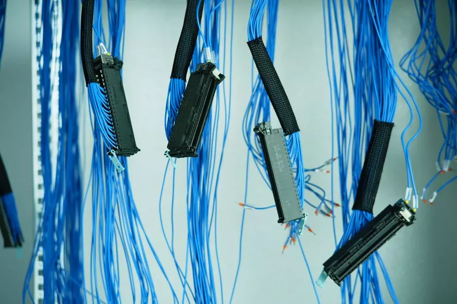
The single most-cited artifact in any monitoring RFP is a parameter table that maps each online analyzer to its regulatory discharge limit and a defensible alarm setpoint. The table below covers the parameters a 500-50,000 m³/day industrial plant typically monitors online, with EPA 40 CFR Part 133 (Secondary Treatment standards for POTWs and equivalent industrial permits), EU Urban Waste Water Directive 91/271/EEC Annex I, and China GB 18918-2002 Grade 1A used as benchmark limits. Where the regulatory citation differs, the most common industrial-permit value is shown.
| Parameter | Online sensor type | Typical regulatory limit (mg/L or as noted) | Pre-alarm setpoint (80%) | Critical alarm setpoint (95%) | Suggested response time |
|---|---|---|---|---|---|
| pH | Glass electrode with reference | 6.0–9.0 SU | 6.2 / 8.8 SU | 6.05 / 8.95 SU | < 60 s |
| Dissolved oxygen (aeration basin) | Optical or membrane | 2.0 mg/L min (process target) | 1.6 mg/L | 1.1 mg/L | < 60 s |
| ORP (anoxic zone) | Platinum electrode | -100 to -50 mV (process) | -80 mV | -55 mV | < 120 s |
| TSS | Optical scattering | 30 mg/L (EPA secondary) | 24 mg/L | 28.5 mg/L | < 5 min |
| Turbidity | Nephelometric | — (trend only; correlates to TSS) | +20% baseline | +50% baseline | < 5 min |
| Conductivity | 4-electrode | 2,000 µS/cm (typical industrial) | 1,600 µS/cm | 1,900 µS/cm | < 5 min |
| Flow | Magnetic or ultrasonic | Site-specific (m³/h) | ±15% daily mean | ±30% daily mean | < 60 s |
| COD | UV-Vis spectrophotometric | 125 mg/L (EU sensitive areas) | 100 mg/L | 119 mg/L | < 15 min |
| NH3-N | UV-Vis or ISE | 10 mg/L (EU UWWTD) | 8 mg/L | 9.5 mg/L | < 15 min |
| Total phosphorus | Online colorimetric | 2 mg/L (EU sensitive areas) | 1.6 mg/L | 1.9 mg/L | < 30 min |
| Total nitrogen | Online digestion + colorimetric | 15 mg/L (EU UWWTD) | 12 mg/L | 14.25 mg/L | < 30 min |
| Temperature | RTD or thermistor | < 35–40 °C (receiving-water protection) | 32 °C | 34 °C | < 5 min |
Modern online UV-Vis spectrophotometric analyzers for COD and NH3-N are now accurate to within ±5% of laboratory values across a 1-1,000 mg/L range, which means the data is suitable for compliance-grade logging rather than just trend monitoring. Process baselines are well established in the literature: impedance-spectroscopy work on industrial wastewater (Springer, 2023) reports 89% COD removal and 73% BOD₅ removal as the performance envelope an effective monitoring system should be protecting, not chasing after the fact.
Three Deployment Architectures: SCADA, Cloud IIoT, and Hybrid
Once the four-layer architecture is clear, the procurement question collapses to: which deployment pattern fits the brownfield or greenfield plant in front of you? The three realistic options for industrial wastewater are summarized below.
| Architecture | Best fit | CAPEX per site (USD) | Recurring OPEX | Deployment time | Key limitation |
|---|---|---|---|---|---|
| A — Extend existing SCADA | Brownfield with working Rockwell/Siemens/Schneider PLCs | $8,000–$45,000 | Telecom $50–$200/mo | 2–4 weeks | Dashboard features limited by what the SCADA exposes |
| B — Cloud-native IIoT | Greenfield plants or multi-site operators wanting standardized dashboards | $5,000–$25,000 | SaaS $200–$800/mo | 1–3 weeks | Vendor lock-in, data residency for EU/China operations |
| C — Hybrid | Regulated facilities (chemical, pharma, petrochemical) that cannot move control logic to the cloud | $15,000–$80,000 | Telecom + SaaS $300–$1,200/mo | 4–8 weeks | Higher integration cost; two systems to maintain |
Architecture A leaves the on-prem SCADA as system of record, adds a cellular or Ethernet gateway, and pushes tag data to a cloud historian for trending and alarm push. It is the lowest-risk retrofit and the right answer for most plants with a SCADA installed after 2010. Architecture B replaces the proprietary SCADA with a vendor-managed IIoT stack — gateway plus cloud SaaS — and is the right answer for greenfield builds or multi-site operators who want identical dashboards at every site. The trade-off is vendor lock-in and the need to verify data residency if you operate in the EU (GDPR) or China (PIPL); a deployment in a single jurisdiction can usually satisfy local data-residency requirements with a regional cloud region, but multi-jurisdictional operators should negotiate contractual data-localization up front. Architecture C keeps the on-prem SCADA as the control system of record and uses the cloud layer purely for trending, alarm push, and multi-site aggregation. It is the most common 2026 retrofit for chemical, pharmaceutical, and petrochemical sites where control logic cannot legally leave the plant network.
The decision rule that covers 80% of RFPs in 2026: if you already have a working SCADA, choose A or C; if you are building new and have fewer than 5 sites, choose B; if you operate 5 or more sites and need centralized compliance reporting, choose C.
Real-World Components and Protocols You Will Specify
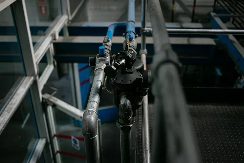
The sensor-side bill of materials is straightforward. pH and DO probes from Hach, Endress+Hauser, or Sensorex with integrated 4-20 mA plus Modbus transmitters are the default; probe lifespan runs 12-24 months in clean municipal-strength wastewater and 3-6 months in oily or high-TDS industrial streams, so the OPEX model should assume a 50% replacement rate per year on the harshest service. On the gateway side, industrial 4G LTE routers from Sierra Wireless, HMS Anybus, or Invendis iRoute handle Modbus TCP to MQTT conversion, and field-bus networking at this layer is well documented in industrial deployments such as the Hawassa Industrial Park power-monitoring project, which is a useful reference architecture for plant-side network design.
On the cloud side, specify a time-series database (InfluxDB or AWS Timestream), a visualization layer (Grafana for open-stack, Ignition Perspective for plant-engineer familiarity), an alarm engine (Node-RED for rule flexibility or vendor SaaS for support), and a notification path (Twilio for SMS, SendGrid for email). Insist on open standards: Modbus TCP/RTU for sensor integration, MQTT for cloud transport, OPC UA for SCADA-to-cloud bridging, and REST API for ERP and CMMS data exchange. If a vendor cannot expose tag data via OPC UA or a documented REST API, the platform will not survive a multi-vendor environment, and you should walk away. Plants integrating remote monitoring with a PLC-controlled automatic chemical dosing skid typically specify OPC UA specifically so dosing interlocks can be wired directly into the alarm engine without a custom protocol converter.
OPEX Impact: What Remote Monitoring Actually Saves
The cost story has to be defensible in front of a CFO, which means the savings are decomposed into two lines and benchmarked against a per-m³ overhead. The two largest savings are: (a) reduced unscheduled site visits, where 60-80% reductions translate to 200-400 avoided visits per year on a 24/7 site at $150-$400 per visit, giving $30,000-$160,000 in annual savings; and (b) faster excursion response preventing 1-3 permit-violation events per year at $10,000-$100,000 per event in fines, cleanup, and reporting overhead. Combined, the lower bound of the savings envelope is around $40,000 per year on a small plant and the upper bound is well over $400,000 on a large, multi-site, high-risk operation.
The per-m³ cost model that should sit inside every monitoring budget is shown below, built from four cost lines against typical industrial wastewater treatment OPEX of $0.40-$2.10 per m³. Telemetry dominates the recurring OPEX only on the smallest sites, while sensor replacement dominates on the largest.
| Cost line | Range (USD per m³ treated) | Basis |
|---|---|---|
| Cellular / telecom | $0.0003–$0.001 | 4G LTE link, 1-min tag push |
| Cloud SaaS / historian | $0.002–$0.01 | Vendor pricing per tag per month |
| Gateway maintenance | $0.01–$0.05 | 5-yr amortized hardware + support |
| Sensor replacement | $0.02–$0.08 | Probes + reagents + calibration labor |
| Total monitoring overhead | $0.04–$0.18 per m³ | 2-10% of typical treatment OPEX |
The headline 20-40% OPEX reduction figure applies to plants with baseline OPEX above $0.50 per m³ where labor is the dominant cost. Small decentralized plants see lower percentage savings but the same absolute chemistry-related savings (prevented chemical overdoses, avoided polymer waste, recovered aeration energy) because those benefits are largely independent of site size. The broader market context reinforces the timing: the digital-water segment is valued above $35B with a 9-12% CAGR to 2030, and smart metering and IIoT are the two largest investment categories inside it. For a deeper OPEX breakdown against treatment-line costs, see the wastewater treatment plant operating cost per m³ in 2026 reference, and for the market-sizing backdrop, the digital water market forecast to 2030.
Frequently Asked Questions
What does a remote monitoring system for an industrial wastewater plant actually include? A four-layer stack — field sensors, PLC or RTU, industrial gateway, and cloud or on-prem SCADA with mobile dashboards — typically priced at $8,000-$80,000 CAPEX per site depending on sensor count and whether you extend an existing SCADA, deploy cloud-native IIoT, or build a hybrid architecture.
What alarm thresholds should we set for EPA and EU compliance? Use an 80% pre-alarm and a 95% critical alarm against the permit limit. For EPA 40 CFR Part 133 this means a 30 mg/L TSS pre-alarm at 24 mg/L, a COD pre-alarm scaled to your specific industrial permit, and pH pre-alarms at 6.2 and 8.8 SU. For EU UWWTD 91/271/EEC sensitive areas, the 10 mg/L NH3-N pre-alarm sits at 8 mg/L and the 125 mg/L COD pre-alarm at 100 mg/L.
How much OPEX does remote monitoring actually save? Industry deployments show 20-40% total OPEX reduction and 60-80% fewer unscheduled site visits. The total monitoring overhead runs $0.04-$0.18 per m³ against typical treatment OPEX of $0.40-$2.10 per m³, so the payback is usually under 18 months once avoided violations and labor savings are included.
How long does deployment take and which architecture should we choose? Two to six weeks is typical. Extend the existing SCADA if it is functional and younger than 10 years; choose cloud-native IIoT for greenfield builds with fewer than 5 sites; choose a hybrid architecture if you operate 5+ sites, run regulated chemical or pharmaceutical processes, or cannot move control logic off-prem.
What are the cybersecurity and data-residency requirements? Specify ISA/IEC 62443 zone-and-conduit segmentation, TLS 1.3 or IPsec VPN between gateway and cloud, and role-based access with audit logging. For EU operations, confirm GDPR-compliant data residency in a regional cloud; for China operations, confirm PIPL compliance and that the cloud region is mainland-China-hosted.
Related Equipment
- MBR membrane bioreactor system — specifications, capacity range, and technical data