Why Traditional Control Struggles in Modern WWTPs
Aeration blowers in municipal and industrial activated-sludge plants consume 40–60% of total electrical OPEX, yet most of that energy is spent holding a fixed dissolved-oxygen (DO) setpoint that ignores diurnal load swings, storm events, and batch discharges from upstream processes (Vanrolleghem 2025 framing of the prediction-vs-control gap). Fixed-DO control is a steady-state solution applied to a fundamentally non-steady process: influent ammonia loadings to a typical 20,000 m³/d plant can vary 3–5× between 02:00 and 14:00, and rule-based PID loops cannot anticipate the swing—they only react after the DO has already dropped. The result is over-aeration during low-load periods (wasted kWh) and under-aeration during peaks (effluent ammonia excursions, the most common 3 a.m. compliance failure mode engineers cite as motivation for pilots). Imen et al. (Johns Hopkins, 2023) identify process uncertainty as the root reason classical control underperforms and recommend probabilistic ML methods as the remedy. This recommendation is now technically feasible because edge inference hardware and OPC-UA bridges have closed the latency gap that kept ML in the lab for the last decade.
ML Model Types That Actually Run Closed-Loop in WWTPs
Four model families have moved from publication to production in operating WWTPs between 2023 and 2026, each mapping to a specific control problem. Supervised regression—ANN, XGBoost, and Random Forest—is the default for effluent quality prediction and soft sensor wastewater applications, where a lab-measured parameter (NH4-N, NO3-N, BOD, COD) is inferred from cheaper online signals (Aparna 2024, Liu 2024, Singh 2023). Time-series deep learning (LSTM, GRU, temporal convolutional networks) handles influent load forecasting with 1–6 hour horizons, which enables feedforward aeration control optimization; the leading case is Xie et al. 2024 (Water Res. 250, 121092), a hybrid deep-learning architecture that improved real-time effluent quality prediction accuracy by 18–25% over feature-engineered baselines. Reinforcement learning (DQN, PPO, SAC) combined with Bayesian optimization enables self-adaptive multi-objective control that simultaneously minimizes energy, effluent ammonia, and chemical cost without a pre-tuned setpoint curve. Hybrid physics-informed models (e.g., the variation sliding layer in Wang et al. 2023, Water Res. 246, 120676) embed process knowledge into the feature layer, which is why Wang's intelligent aeration control framework is the most-cited aeration-specific deployment in 2024–2026 literature.
| Model Family | Typical Control Loop | Inference Latency | Training Data Need | Reference Deployment |
|---|---|---|---|---|
| Supervised regression (ANN, XGBoost, RF) | Soft sensor for NH4-N/NO3-N; advisory effluent prediction | 50–200 ms | 6–12 months, ≥15 min cadence | Aparna 2024, Singh 2023 |
| LSTM / GRU time-series | Influent load forecasting 1–6 h ahead; feedforward aeration bias | 100–400 ms | 12+ months, seasonal coverage | Xie et al. 2024 |
| Reinforcement learning (DQN, PPO) | Multi-objective aeration + chemical cost balancing | 10–100 ms (policy lookup) | Sim + 3–6 mo plant fine-tune | Consensus synthesis, 2024 |
| Physics-informed hybrid (variation sliding layer) | Aeration DO setpoint, airflow scheduling | 80–250 ms | 6–9 months | Wang et al. 2023 |
ML vs Rule-Based Control: When Each Wins
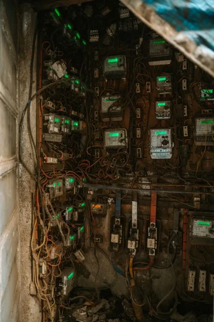
Rule-based control remains effective for a specific subset of low-complexity loops. PID, fuzzy logic, and lookup-table strategies still win for single-input loops with low process memory: pH trim, chlorine residual, and polymer dose on relatively constant TSS influent. They also win where regulators demand fully explainable setpoint logic—where every setpoint change must be traceable to a written operating procedure. ML wins on loops with multi-variable coupling and high load variance: aeration with simultaneous DO, NH4-N, and airflow interaction; polymer dosing on a variable-TSS influent; and predictive sludge recycle driven by SVI trends. The 2024–2026 deployment pattern, documented in AquaFlowNet (2024) and the Vanrolleghem 2025 review, is hybrid: an ML model generates a recommended setpoint or feedforward bias every 1–5 minutes, and the existing PID executes the final actuator command. This preserves the safety and auditability of PID while capturing the load-anticipation value of ML. For a deeper comparison of how ML outputs surface inside operator dashboards, see the wastewater KPI dashboard architecture guide.
| Decision Dimension | Rule-Based (PID / Fuzzy / Lookup) | Machine Learning | Hybrid (ML → PID) |
|---|---|---|---|
| Adaptability to load swings | Low (reactive only) | High (predictive) | High |
| Commissioning time | Days | 6–12 weeks | 8–14 weeks |
| Data requirement | None historical; tuning constants | ≥6 months clean, all seasons | ≥6 months clean, all seasons |
| Interpretability for regulators | Full (equations) | Partial (SHAP, feature importance) | Full for PID layer, partial for ML bias |
| OPEX savings vs fixed setpoint | 0–5% | 10–30% (aeration) | 10–25% (aeration) |
| O&M skill needed | Process engineer | Process engineer + data scientist | Process engineer + part-time DS support |
Integration Architecture: ML Into an Existing SCADA/PLC Plant
Most plants in 2026 execute a three-layer stack integrated with existing Allen-Bradley ControlLogix, Siemens S7-1500, or Schneider M580 hardware without requiring PLC replacement. Layer 1 is the existing PLC executing deterministic control at sub-100 ms cycle time; it remains in charge of all hardwired safety interlocks and final actuator output. Layer 2 is an industrial PC or edge gateway (e.g., Beckhoff CX, Siemens IPC, or a ruggedized x86 box) that hosts the trained ML model and runs inference at 100–300 ms cadence. Layer 3 is an on-prem server or private cloud instance that handles model training, drift monitoring, and version management. The two practical bridges between Layer 2 and Layer 1 in 2026 retrofits are OPC-UA (preferred for new plants, supports Pub/Sub and structured writes) and Modbus TCP (preferred for brownfield sites where OPC-UA server licensing is cost-prohibitive). Closed-loop aeration needs an end-to-end inference-to-actuator latency under 200 ms; chemical dosing on slow metering pumps tolerates 1–5 s; advisory-only effluent prediction has no hard latency floor. Sensor minimum viable spec for ML training is DO, NH4-N, NO3-N, TSS, flow, and temperature at ≥15 min cadence with at least 12 months of clean data covering all four seasons—Imen et al. 2023 explicitly flag data quality, not algorithm choice, as the dominant barrier to ML deployment. Chemical dose loops can be retrofitted onto a PLC-controlled chemical dosing skid that exposes OPC-UA write nodes for ML setpoint bias.
Aeration Control With ML: The Highest-ROI Use Case
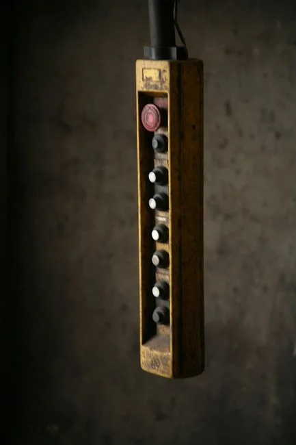
Aeration is the single control loop where the ML business case is most defensible due to the large energy denominator. Across the peer-reviewed literature from 2023 to 2026—Wang et al. 2023, Xie et al. 2024, and the Consensus synthesis of 12 deployment studies—ML-based aeration reports 10–30% blower energy reduction versus constant-DO setpoints, with a central tendency around 18% for plants with high influent variability. On a 20,000 m³/d industrial WWTP drawing aeration blowers at roughly 250 kW continuous, that 15–25% reduction translates to $40,000–$180,000/year in 2026 industrial electricity tariffs (US $0.08–0.12/kWh, 8,000 operating hours). The downstream benefit is often larger than the direct energy saving: stable ML-controlled DO tightens sludge age variability, which directly improves membrane flux stability on an MBR membrane bioreactor system and reduces the polymer dose required for sludge dewatering. Engineers scoping ML pilots at chemical-industrial sites should also review the AI process control for chemical wastewater plants guide, which documents the same control patterns applied to higher-strength feeds with toxicity events.
90-Day ML Pilot Framework for a Single Control Loop
Engineers evaluating funding for full deployment should use a pilot scoped to a single loop with explicit go/no-go gates. Weeks 1–2 — data audit: confirm sensor coverage matches the minimum viable spec (DO, NH4-N, NO3-N, TSS, flow, temperature at ≥15 min cadence), validate calibration records, and verify at least 6 months of clean historical data. Data gaps discovered here are the most common reason pilots stall. Weeks 3–6 — shadow mode: train the offline model on the audited dataset, then connect it to the SCADA historian in write-disabled mode; the ML outputs recommended setpoints every 1–5 minutes, but the PLC continues executing the existing PID. Compare ML recommendations against PID outputs offline to quantify the theoretical energy delta. Weeks 7–10 — bounded closed-loop trial: allow the ML output to bias the PID setpoint within a hard ±15% clamp, with deviation alarms that fall back to PID-only control if exceeded. Weeks 11–13 — full closed-loop on a defined operating envelope: release the clamps for a documented envelope (influent flow range, NH4-N load range, temperature window) and capture the energy, chemical, and effluent quality delta against the 12-week pre-pilot baseline. For plants that want to extend the same framework to influent forecasting, the AI influent load prediction guide covers the upstream forecasting layer that feeds the aeration bias.
Frequently Asked Questions
How much historical data do I need before an ML aeration pilot is worth starting?
At least 6 months of clean data covering one full seasonal cycle, with DO, NH4-N, NO3-N, TSS, flow, and temperature sampled at 15-minute or tighter cadence; Imen et al. 2023 identified insufficient data as the primary deployment barrier across surveyed utilities.
What inference latency is acceptable for closed-loop aeration control?
End-to-end from sensor read to actuator write must stay under 200 ms; this is achievable with edge inference on industrial PCs and OPC-UA Pub/Sub to the PLC, as documented in Wang et al. 2023.
What does an