Why Manual Dosing Breaks Down in Paper Mills
Manual coagulant dosing in a paper mill is essentially an open-loop guess anchored to a once-per-shift grab sample and a fixed setpoint. That setpoint is almost always wrong within hours, because paper-mill influent is highly variable: typical COD swings from 1,000 to 5,000 mg/L, pH between 6.5 and 9, and color that tracks lignin release through the bleach sequence and changes with furnish, grade transitions, and wash-ups (hydrochemix, 2026). A dose sized for the average load over-doses during low-load periods, wasting coagulant and pumping extra solids into the press, and under-doses during spike events, pushing color and COD past the discharge consent.
Frame the same problem as a control engineer and the failure mode is obvious. Per Hahn's boundary-condition framework for coagulant dosing, two conditions must hold simultaneously: the coagulant species must form in a homogeneous concentration field, and the in-situ-formed species must reach the colloid surface before the destabilization step is over (Hahn, 1992). Static, timer-based dosing cannot satisfy either condition when the influent itself is non-stationary. The cost driver behind the engineering problem is coagulant spend plus downstream sludge handling, and Polyaluminum Chloride (PAC) already produces 30-50% less sludge than alum, so the choice of coagulant compounds with how well the dose is modulated (hydrochemix, 2026). A PLC-controlled automatic chemical dosing system is the hardware layer that makes modulation possible; the AI layer decides what to set the pump to.
What AI Optimization of Chemical Dosing Actually Does
AI optimization of chemical dosing in paper manufacturing is a closed control loop in which online sensors drive a machine-learning model that sets the metering-pump stroke rate in near real time. The signal path is: streaming pH, turbidity, color or UV254, TOC where available, and influent flow are aggregated into 1-5 minute features; the model — typically a random forest, gradient-boosted regression, or LSTM for time-series — predicts the minimum dose that holds color and COD below their setpoints; the prediction is written as a 4-20 mA or Modbus setpoint to the metering pump. The loop is updated every 1-5 minutes rather than once per shift.
Three control layers are usually stacked rather than chosen between. (1) Feedforward acts on influent flow and load, adjusting dose immediately when hydraulic loading changes. (2) Feedback trims the dose against measured effluent quality, correcting for model bias. (3) Model predictive control uses the trained model as the primary controller, with feedforward and feedback as overrides. The result is dose setpoints that track the influent instead of lagging it by hours.
The savings case is grounded in adjacent work. Computational modeling at the Stora Enso Skoghall mill — a combined MBBR and aerated lagoon treating pulp-and-paper wastewater — found that lowering dissolved oxygen from 3 to 2 mg/L in the MBBR and using a Hyperclassic aerator delivered a 48.5% OpEx reduction and a 60% energy reduction with no loss of treatment efficiency (Sorlini et al., 2023, Journal of Water Process Engineering, vol. 56). The same closed-loop principle applied to coagulant and flocculant dosing typically yields 10-20% chemical savings plus a measurable reduction in sludge volume, with smaller capital changes than a biological-stage retrofit. AI here does not replace the jar test; it consumes jar-test data as training labels and uses bench tests to validate the model after every retraining cycle.
Sensor Stack and Data Inputs for an AI Dosing Loop
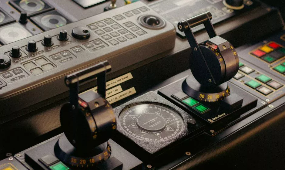
The minimum instrumentation package for an AI coagulant loop on a paper-mill clarifier or DAF is narrower than vendors suggest. Required inputs are influent flow, pH, temperature, turbidity, streaming UV254 or color at 254 nm, and — if already installed — a TOC or COD probe on the clarifier feed. Desired but optional inputs are pump stroke feedback, sludge blanket level, and the DAF or clarifier solids loading rate. A streaming UV254 sensor is the single highest-value addition for a mill currently dosing on flow and pH alone, because lignin-derived color correlates strongly with UV absorbance and responds in seconds to grade changes.
Data quality is the limiting factor. High-TSS streams foul probes within hours; automatic cleaning cycles referenced in ultrafiltration systems rated for up to 300 ppm turbidity are the same engineering principle applied at smaller scale to in-pipe optical sensors (HydropureWater field data, 2026). Sampling cadence matters: 1-second raw signals are smoothed into 1-5 minute features, and the model never sees the raw signal. Engineers specifying a package in 2026 should also plan for a redundant pH probe and a streaming color or UV254 sensor with built-in air-blast cleaning — a single fouled sensor will silently bias the dose for hours before the alarm fires.
| Signal | Sensor type | Typical range, paper-mill influent | Update cadence | Notes for AI loop |
|---|---|---|---|---|
| Influent flow | Magnetic flowmeter | 500-5,000 m³/day | 1 s | Primary feedforward input |
| pH | Glass electrode with ATC | 6.5-9.0 | 1 s, averaged 1 min | Defines PAC/PFS activity window |
| Temperature | RTD | 25-55 °C | 10 s | Required for pH compensation |
| Turbidity | Scattered-light, 90° | 200-1,500 NTU | 10 s, averaged 1 min | Auto-clean cycle mandatory |
| Streaming UV254 / color | In-line UV absorption | 0.5-6.0 abs/cm | 1 s, averaged 1-5 min | Highest-value color proxy |
| TOC (where installed) | Online combustion or UV | 300-2,500 mg/L | 5-15 min | Strongest load proxy, slow response |
| Pump stroke feedback | Potentiometer / encoder | 0-100% stroke | 1 s | Closes the inner control loop on the pump |
This is the same signal stack that feeds dissolved air flotation systems used after coagulant dosing; the AI controller simply becomes the dose setpoint source rather than a manual operator.
Dosing Parameters and Expected Removal Performance
The dose ranges below are taken from operating data in paper-mill chemical treatment programs and are the bands an AI model should be initialized against (hydrochemix, 2026). Manual dosing rarely holds the upper end of these bands consistently because the operator sets a dose once and rides it through the shift; AI dosing is differentiated by the ability to track the upper end of each band within minutes of a load change. The failure mode the model must guard against is the bleach-plant or black-liquor spill, where a 3-5× COD excursion in under an hour will saturate a static dose. Anomaly-detection logic on the streaming UV254 signal is the standard guard.
| Treatment stage | Chemical | Typical dose range | Expected removal | AI loop behavior |
|---|---|---|---|---|
| Primary coagulation | PAC (polyaluminum chloride) | 50-300 mg/L as Al₂O₃ | 60-90% TSS, fiber recovery | Feedforward on flow + solids, feedback on turbidity |
| Primary flocculation aid | Anionic PAM | 0.5-3 mg/L | Improves settling/clarity | Trim against streaming turbidity |
| Tertiary color removal | PAC | 80-250 mg/L as Al₂O₃ | 70-90% residual color | Feedback on UV254/color, 1-5 min updates |
| Tertiary COD polishing | PFS (polyferric sulfate) | 40-150 mg/L as Fe | 30-60% residual COD | Blend with PAC, target upper band |
| Blend polishing | PAC:PFS at 70:30 to 50:50 | 100-250 mg/L total | Combined COD + phosphate polishing | Model selects ratio per shift |
| Sludge conditioning | Cationic PAM | 3-10 kg/ton dry solids | Improved cake solids, lower polymer demand | Controlled by dewatering press feed |
For a 10,000 m³/day recycled-fiber packaging mill, holding the upper end of the tertiary color band (90% rather than 70%) translates directly into a lower effluent color number and a smaller monthly coagulant spend, because the dose is no longer padded for the worst expected load (hydrochemix, 2026).
Closing the Loop: From Model to Metering Pump
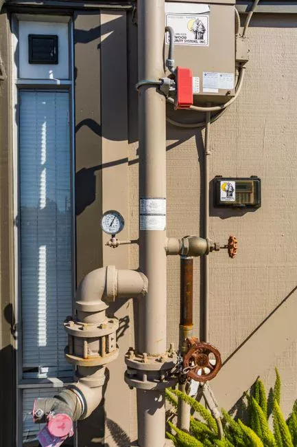
The most common engineering concern in 2026 is not the model — it is the last meter of wire from the controller to the pump. The standard architecture is an edge device (industrial PC, PLC with inference runtime, or DCS controller) running the model on a 1-5 minute cycle and writing the dose setpoint to the pump over 4-20 mA, Modbus RTU, or Modbus TCP. The pump's variable-frequency drive or stroke controller accepts the setpoint directly; no custom protocol stack is required. PLC-controlled automatic chemical dosing systems are pre-wired for this signal chain, with a pre-engineered I/O map that exposes the dose setpoint, stroke feedback, and alarm contacts as standard tags.
The safety layer is non-negotiable. Hard-coded minimum and maximum dose limits clamp the AI output to a band the operations team has approved; pump stroke-rate alarms fire if the requested dose would push the pump beyond its reliable range; a watchdog timer drops the controller to a last-good setpoint if any sensor signal goes out of range or fails to update. Stroke feedback is essential because pump output is non-linear near the endpoints of the stroke and shifts as the chemical's viscosity changes with temperature and age. A model that assumes 60% stroke equals 60% flow will drift out of calibration within a week of a seasonal temperature swing.
ROI and OpEx Impact of AI-Optimized Dosing
The financial case is anchored in published mill data and conservative field estimates. The Stora Enso Skoghall study reported 48.5% OpEx and 60% energy reductions from a closed-loop aeration and nutrient-dosing optimization, with co-benefits of approximately 100 t CO₂-eq/yr and 140 kg PO₄³⁻-eq/yr (Sorlini et al., 2023). A coagulant-focused AI retrofit delivers a smaller headline number because chemical spend is only one line item, but it is realized in months rather than years: 10-20% chemical savings is a realistic band when the model is initialized from existing jar-test data and the dose loop is closed against live UV254 and flow (HydropureWater field data, 2026).
Sludge handling is the second savings line and is often the larger one. PAC generates 30-50% less sludge than alum, and AI control further reduces sludge volume by eliminating the chronic over-dose that manual control accumulates as a safety margin (hydrochemix, 2026). Lower sludge volume means lower polymer demand on the dewatering press, fewer truck loads, and lower disposal cost. For a mill spending more than $200K/yr on coagulant, a 12-24 month payback is achievable; mills with higher loads or stricter color consents typically see the payback in under 18 months because the avoided non-compliance risk is non-trivial. The same control principles covered in the pulp and paper wastewater aeration system design guide apply to the dosing side of the treatment train.
| Line item | Manual dosing baseline | AI-optimized dosing | Saving band |
|---|---|---|---|
| Coagulant spend (PAC, PFS) | 100% | 80-90% | 10-20% |
| Flocculant (PAM) demand | 100% | 85-95% | 5-15% |
| Sludge volume to dewatering | 100% | 70-85% | 15-30% |
| Dewatering polymer (cationic PAM) | 100% | 85-95% | 5-15% |
| Color excursions past consent | Baseline | 50-80% reduction | Compliance risk |
| Jar-test frequency | Weekly to monthly | Monthly, plus continuous model output | Labor savings |
Selecting an AI Dosing System in 2026: A Buyer Checklist
The 2026 market separates into two categories: vendors selling an "AI" label over a rule-based controller, and vendors with a deployable loop that closes against real sensors on a real pump. The checklist below is the minimum a paper-mill engineer should run a vendor through before signing a PO.
- Model transparency. Can the operations team inspect feature importance, see which sensor drove each setpoint change, and override any single input? Black-box models that only the vendor can interpret are a 5-year lock-in risk.
- Edge vs cloud inference. Paper-mill DCS networks often run air-gapped. Confirm the model runs on an edge device or PLC, with cloud connectivity as an option, not a requirement.
- Cybersecurity. ISA/IEC 62443 compliance, signed firmware, and role-based access are no longer optional for systems that write setpoints to a pump.
- Integration with existing DCS. OPC UA, Modbus, or 4-20 mA into the existing control system, with documented tag maps. A standalone vendor box that operators must log into separately will be bypassed within a month.
- Vendor-supplied jar-test campaign. The model needs labeled data from the actual mill, not a generic training set. A 2-4 week on-site campaign with bench tests at the planned dose range is the standard.
- Defined retraining cadence. Quarterly at minimum, with an explicit trigger for unplanned retraining after a major grade change or process upset.
- Hardware criteria. Skid pre-wiring, chemical compatibility (PAC and PFS are acidic and corrosive; PAM is often viscous at low temperature), and stroke feedback on every pump.
- Common pitfalls to reject. "AI" with no live sensor feedback; models that only retrain offline and cannot respond within a shift; dose outputs with no hard-coded upper and lower limits; sensors without auto-clean.
Cross-check pH-control integration against the pH adjustment system maintenance guide — pH is a primary input to the AI loop, and a poorly maintained pH probe will silently bias the model.
Frequently Asked Questions
What dose of PAC or PFS should a paper mill expect for tertiary color and COD removal?
Tertiary dosing typically falls in 80-250 mg/L as Al₂O₃ for PAC and 40-150 mg/L as Fe for PFS, with blend ratios from 70:30 to 50:50 PAC:PFS for combined COD and phosphate polishing. AI control targets the upper end of the 70-90% color and 30-60% residual COD removal bands more consistently than manual dosing (hydrochemix, 2026).
How much can AI dosing realistically save a paper mill per year?
A coagulant-focused AI retrofit typically delivers 10-20% chemical savings, 15-30% lower sludge volume, and 5-15% lower flocculant demand, with 12-24 month payback for mills spending more than $200K/yr on coagulant. The Stora Enso Skoghall study reported a 48.5% OpEx reduction on the aeration and nutrient side, which sets the ceiling for what closed-loop process control can deliver on a paper-mill WWTP (Sorlini et al., 2023).
Does AI dosing replace jar testing?
No. AI dosing augments jar testing: bench tests supply the labeled training data the model is initialized on, validate model behavior at startup, and are run monthly to confirm the model is not drifting. The AI loop runs between jar tests, on a 1-5 minute update cadence, and catches the grade-change and wash-up spikes that weekly jar tests miss by hours.
What is the minimum sensor package to specify in 2026?
Influent flow, pH with automatic temperature compensation, turbidity with auto-clean, and a streaming UV254 or color probe. A TOC analyzer is a strong addition if the budget allows, and pump stroke feedback is required on every pump the AI writes to (HydropureWater field data, 2026).