Here's the edited HTML with light-touch corrections:

Why Wastewater Plants Need Predictive Maintenance: The Hidden Costs of Reactive Repairs

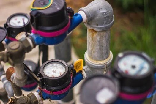
At 2:17 AM on a Tuesday, the lead operator at a Midwest food processing plant received an urgent alert: "DAF system motor bearing failure imminent." By 3:03 AM, the dissolved air flotation unit had seized, forcing an emergency shutdown of the entire pretreatment line. The plant lost 48 hours of production—$120,000 in revenue—while crews replaced the $18,000 bearing assembly and recalibrated the system. This scenario occurs regularly. According to the EPA's 2023 Industrial Water Survey, unplanned downtime in wastewater treatment plants costs operators $1,500-$5,000 per hour, with 62% of failures occurring in critical equipment like pumps, DAF systems, and MBR membranes.

Reactive maintenance disrupts operations while eroding profitability, compliance, and equipment lifespan. For industrial wastewater plants, the financial impact compounds across multiple systems:

• DAF systems: Bearing failures in motors or air dissolution tanks cost $12,000-$25,000 per incident, with 3-5 days of downtime for repairs. Vibration analysis can detect early-stage bearing wear (0.1g acceleration at 1x RPM) 4-6 weeks before failure.
• MBR membranes: Fouling reduces flux by 30-50% before visible performance drops, increasing energy costs by 2-3x. Acoustic sensors can detect fouling at 20-40 kHz frequencies 2-3 weeks before operational impact.
• Chemical dosing pumps: Diaphragm ruptures and valve clogging account for 12-18% of treatment plant emergencies, with average repair costs of $8,500. Pressure sensors (0-10 bar range) can identify blockages at 15% deviation from baseline flow rates.
• Sludge dewatering equipment: Belt press mistracking causes 28% of unplanned downtime in municipal plants, with each incident costing $5,000-$15,000 in repairs and lost capacity.

Regulatory risks add to the burden. UK Water Industry Research (2024) found that plants relying on reactive maintenance experience 40% more non-compliance incidents due to equipment failures during peak loads. For example, a failed aeration blower can trigger dissolved oxygen violations within 30 minutes, while a malfunctioning chemical dosing pump may cause pH excursions in under an hour.

Equipment Type	Common Failure Mode	Average Downtime	Direct Repair Cost	Indirect Costs (Production Loss + Regulatory)
DAF System (Motor/Bearing)	Bearing wear, seal failure	3-5 days	$12,000-$25,000	$50,000-$150,000
MBR Membrane	Fouling, integrity loss	1-3 days	$8,000-$20,000	$30,000-$90,000
Chemical Dosing Pump	Diaphragm rupture, valve clog	4-12 hours	$3,000-$8,500	$10,000-$40,000
Sludge Dewatering (Belt Press)	Belt mistracking, roller failure	6-24 hours	$5,000-$15,000	$20,000-$80,000
Aeration Blower	Bearing failure, impeller damage	1-2 days	$10,000-$30,000	$40,000-$120,000

How Predictive Maintenance Works in Wastewater Treatment: From Sensors to Actionable Alerts

Predictive maintenance converts wastewater equipment from black boxes into transparent, data-driven assets. The system operates on three pillars—data collection, analysis, and action—each adapted to the unique challenges of industrial wastewater treatment. Wastewater systems face high moisture, corrosive chemicals, and biological fouling, requiring specialized sensor configurations and analytical models.

Data Collection: Sensor Technologies for Wastewater Environments

Wastewater equipment requires sensors that withstand harsh conditions while providing high-fidelity data. Key technologies include:

• Vibration Sensors: Triaxial accelerometers (10-1,000 Hz range, 0.1g sensitivity) detect bearing wear, misalignment, and imbalance in pumps and blowers. For example, a 1x RPM spike at 0.3g indicates early-stage bearing wear in a DAF system motor, while 2x and 3x RPM harmonics suggest misalignment.
• Oil Analysis: Online particle counters (ISO 4406) and viscometers monitor gearbox and compressor health. Alarm thresholds for wastewater applications are typically set at >16/14/11 for particle count, with wear metals (Fe, Cu, Pb) tracked via trend analysis. A 20% increase in iron particles over 30 days signals impending gearbox failure.
• Acoustic Sensors: Ultrasonic microphones (20-100 kHz range) detect valve leaks, cavitation, and membrane fouling. In MBR systems, fouling generates a distinct 30-40 kHz signature 2-3 weeks before flux reduction, while cavitation in pumps produces broadband noise at 50-80 kHz.
• Pressure Sensors: Differential pressure transmitters (0-10 bar range) monitor filter clogging, pipe blockages, and membrane integrity. A 15% deviation from baseline pressure in a chemical dosing line indicates valve clogging or diaphragm failure.
• Temperature Sensors: Surface-mounted RTDs and infrared thermometers track motor and bearing temperatures. Alarms trigger at 10°C above normal operating range (e.g., 85°C for a 75°C-rated motor).

Data Analysis: Machine Learning for Wastewater-Specific Failure Modes

Generic predictive maintenance models fail in wastewater applications due to process variability (flow rates, chemical composition, biological load). Wastewater-specific models incorporate:

• Time-Domain Analysis: RMS and peak-to-peak vibration values identify gradual degradation. For example, a 30% increase in RMS vibration over 7 days signals bearing wear in a progressive cavity pump.
• Frequency-Domain Analysis (FFT): Spectral analysis pinpoints failure modes:
  • 1x RPM: Unbalance or misalignment
  • 2x RPM: Looseness or resonance
  • 3x RPM: Bearing defects (ball pass frequency)
  • High-frequency spikes: Cavitation or gear mesh issues
• Oil Condition Monitoring: Trend analysis of wear metals (Fe, Cu, Pb) and contaminants (Si, Na) predicts component failure. A 50% increase in copper particles over 2 weeks indicates bronze bearing wear in a blower.
• Acoustic Pattern Recognition: Machine learning models classify sound signatures for MBR fouling (30-40 kHz), valve leaks (20-30 kHz), and cavitation (50-80 kHz). Models trained on wastewater-specific data achieve 92% accuracy in fouling detection, compared to 65% for generic industrial models.

Actionable Alerts: From Data to Maintenance Decisions

Effective predictive maintenance systems convert data into prioritized maintenance tasks. A typical alert matrix for wastewater plants includes:

Severity Level	Threshold Criteria	Recommended Action	Response Time	Example (Pump Vibration)
Critical	Parameter >90% of failure threshold	Immediate shutdown + emergency repair	<2 hours	Vibration >0.8g at 1x RPM
High	Parameter 70-90% of failure threshold	Schedule repair within 24 hours	24 hours	Vibration 0.5-0.8g at 1x RPM
Medium	Parameter 50-70% of failure threshold	Inspect during next planned maintenance	7 days	Vibration 0.3-0.5g at 1x RPM
Low	Parameter 30-50% of failure threshold	Monitor trend, no immediate action	30 days	Vibration 0.1-0.3g at 1x RPM

For more details on sensor selection and integration, refer to our detailed guide on selecting IoT sensors for wastewater equipment.

Sensor Selection Matrix: Matching Technologies to Wastewater Equipment

Not all predictive maintenance technologies perform equally across wastewater equipment. The optimal sensor configuration depends on failure modes, environmental conditions, and process requirements. This matrix provides engineering specifications for matching technologies to specific equipment types:

Equipment Type	Common Failure Modes	Recommended Sensor Types	Key Parameters to Monitor	Typical Alarm Thresholds
Centrifugal Pumps	Bearing wear, seal failure, cavitation, impeller damage	Vibration (10-1,000 Hz), acoustic (20-100 kHz), pressure (0-10 bar), temperature (RTD)	Vibration (RMS, 1x/2x/3x RPM), cavitation noise, suction/discharge pressure, motor temperature	Vibration >0.3g at 1x RPM, pressure deviation >15%, temperature >85°C
DAF Systems	Motor bearing wear, air dissolution tank leaks, pump cavitation	Vibration (10-1,000 Hz), acoustic (20-100 kHz), pressure (0-6 bar), temperature (RTD)	Motor vibration, tank pressure, pump cavitation noise, motor temperature	Vibration >0.4g at 1x RPM, pressure <2 bar (tank leak), cavitation noise >70 dB
MBR Membranes	Fouling, integrity loss, aeration inefficiency	Acoustic (20-100 kHz), pressure (0-1 bar), flow (0-100 m³/h), DO (0-20 mg/L)	Fouling frequency (30-40 kHz), TMP, permeate flow, aeration DO	Fouling frequency >60 dB, TMP >0.5 bar, flow <80% of baseline
Chemical Dosing Systems	Diaphragm rupture, valve clogging, motor burnout	Pressure (0-10 bar), flow (0-50 L/h), vibration (10-1,000 Hz), temperature (RTD)	Suction/discharge pressure, flow rate, pump vibration, motor temperature	Pressure deviation >20%, flow <90% of setpoint, vibration >0.5g
Sludge Dewatering (Belt Press)	Belt mistracking, roller bearing wear, hydraulic leaks	Vibration (10-1,000 Hz), acoustic (20-100 kHz), pressure (0-100 bar), temperature (RTD)	Roller vibration, belt tracking noise, hydraulic pressure, bearing temperature	Vibration >0.6g at 1x RPM, tracking noise >80 dB, pressure <80% of baseline
Aeration Blowers	Bearing wear, impeller damage, inlet filter clogging	Vibration (10-1,000 Hz), acoustic (20-100 kHz), pressure (0-1 bar), temperature (RTD), oil analysis	Vibration (RMS, 1x/2x RPM), inlet pressure, motor temperature, oil particle count	Vibration >0.5g at 1x RPM, pressure <0.8 bar, temperature >90°C, oil >16/14/11

Sensor Specifications for Wastewater Applications

Wastewater environments demand sensors with specific technical parameters to ensure reliability and accuracy:

Sensor Type	Measurement Range	Accuracy	Environmental Rating	Power Requirements	Data Output	Typical Cost Range
Triaxial Accelerometer	10-1,000 Hz	±5% or 0.01g	IP68	4-20mA or 24V DC	4-20mA, Modbus, OPC UA	$300-$800
Ultrasonic Acoustic Sensor	20-100 kHz	±2 dB	IP67	12-24V DC	4-20mA, Modbus, wireless	$500-$1,200
Differential Pressure Transmitter	0-10 bar	±0.25% FS	IP66	12-36V DC	4-20mA, HART, Modbus	$400-$900
Oil Particle Counter	4-70 µm	±1 ISO code	IP65	24V DC	Modbus, Ethernet	$2,000-$5,000
Surface-Mount RTD	-50°C to 200°C	±0.1°C	IP67	3-5V DC	4-20mA, Modbus	$150-$400

Integration Considerations

Connecting predictive maintenance sensors to existing systems requires careful planning:

• Protocols: Most wastewater plants use 4-20mA for legacy systems, Modbus for PLCs, and OPC UA for SCADA integration. Wireless options (LoRaWAN, NB-IoT) are gaining traction for remote or hard-to-wire equipment.
• Edge Computing: Local processing reduces latency and bandwidth requirements. For example, vibration data from a DAF system motor can be analyzed at the edge, with only alerts sent to the central system.
• SCADA Integration: Predictive maintenance data should be displayed alongside process parameters. For example, vibration trends for a pump can be shown on the same screen as flow and pressure data. Learn more about how to integrate predictive maintenance data with SCADA systems.

Case Example: MBR Fouling Detection

A municipal wastewater plant in California reduced MBR membrane fouling by 40% using acoustic sensors and real-time flux monitoring. The system included:

• 8 ultrasonic acoustic sensors (20-100 kHz range) installed on membrane modules
• Differential pressure transmitters (0-1 bar) to monitor transmembrane pressure (TMP)
• Flow meters (0-100 m³/h) to track permeate flux
• Edge computing device for local data processing

The plant set alarm thresholds at:

• Fouling frequency >60 dB at 30-40 kHz
• TMP >0.5 bar
• Permeate flux <80% of baseline

When fouling was detected, the system triggered an automated cleaning cycle (increased aeration + backpulse) and alerted operators. Over 12 months, the plant reduced chemical cleaning frequency from weekly to biweekly, saving $45,000 in chemicals and extending membrane life by 18 months.

ROI Calculation Framework: Predictive Maintenance Costs vs. Savings for Wastewater Plants

Predictive maintenance serves as both a technical upgrade and a financial strategy. For wastewater plants, the ROI depends on quantifiable savings across downtime, energy, labor, and equipment lifespan. This framework helps operators calculate costs and savings specific to their plant size and equipment mix.

Cost Components

Predictive maintenance requires upfront investment in hardware, software, and integration. Typical costs for a mid-sized plant (500-2,000 m³/day) include:

Cost Component	Description	Typical Cost Range	Notes
Hardware	Sensors, gateways, edge computing devices	$2,000-$15,000	Cost varies by equipment count and sensor types (e.g., vibration vs. acoustic)
Software	Licensing, cloud storage, analytics platform	$5,000-$50,000/year	Cloud-based solutions typically cost $1,000-$5,000/month for mid-sized plants
Installation	Wiring, calibration, integration with existing systems	$3,000-$20,000	Wireless sensors reduce installation costs by 30-50%
Training	Operator and maintenance staff training	$2,000-$10,000	Includes initial training and annual refreshers
Maintenance	Sensor calibration, software updates, data management	$1,000-$5,000/year	Self-cleaning sensors reduce maintenance costs by 20-40%

Savings Components

Predictive maintenance delivers measurable savings across multiple operational areas:

• Reduced Unplanned Downtime: Plants typically achieve 35-50% reduction in unplanned downtime. For a mid-sized plant with 100 hours of annual downtime at $3,000/hour, this translates to $105,000-$150,000 in savings.
• Extended Equipment Life: Predictive maintenance extends asset lifespan by 20-40%. For a $50,000 pump with a 10-year lifespan, this adds 2-4 years of service, saving $10,000-$20,000 in capital expenditure.
• Energy Savings: Optimized operation reduces energy costs by 5-15%. For a plant with $200,000 in annual energy costs, this equals $10,000-$30,000 in savings. For example, detecting fouled MBR membranes early can reduce aeration energy by 20-30%.
• Labor Savings: Predictive maintenance shifts labor from reactive to planned tasks, reducing emergency repair costs by 20-30%. For a plant with $100,000 in annual maintenance labor, this saves $20,000-$30,000.
• Chemical Savings: Optimized dosing reduces chemical usage by 10-20%. For a plant spending $150,000/year on chemicals, this equals $15,000-$30,000 in savings. For example, chemical dosing systems with integrated predictive maintenance sensors can adjust dosing in real-time based on fouling or flow conditions.

ROI Calculation Template

Use this worksheet to calculate ROI for your plant. Example values are provided for a 1,000 m³/day plant with 3 pumps, 1 DAF system, 1 MBR system, and 2 blowers:

Category	Calculation	Example Value	Your Plant
Annual Costs
Hardware	One-time cost	$12,000
Software	Annual licensing	$18,000
Installation	One-time cost	$15,000
Training	One-time cost	$5,000
Maintenance	Annual cost	$3,000
Total First-Year Cost	Sum of all costs	$53,000
Annual Savings
Reduced Downtime	Downtime hours × cost/hour × reduction %	$120,000
Extended Equipment Life	Annualized capital savings	$25,000
Energy Savings	Energy cost × reduction %	$20,000
Labor Savings	Maintenance labor × reduction %	$25,000
Chemical Savings	Chemical cost × reduction %	$20,000
Total Annual Savings	Sum of all savings	$210,000
First-Year ROI	(Savings - Costs) / Costs × 100%	296%
Payback Period	Costs / Annual Savings	3.2 months

Payback Period by Plant Size

ROI timelines vary by plant capacity and equipment complexity:

• Small Plants (100-500 m³/day): 18-24 months. Lower equipment counts reduce hardware costs but limit savings potential.
• Medium Plants (500-2,000 m³/day): 12-18 months. This range offers an optimal balance of cost and savings, with payback often achieved in the first year.
• Large Plants (>2,000 m³/day): 6-12 months. High equipment counts and operational costs drive rapid ROI, often within 6-9 months.

Implementation Roadmap: From Pilot to Full-Scale Predictive Maintenance

Deploying predictive maintenance in a wastewater plant requires a phased approach to minimize disruption and validate results. This roadmap outlines a 6-12 month implementation plan, starting with a pilot program and scaling to full deployment.

Step 1: Equipment Criticality Assessment

Prioritize equipment based on failure frequency, repair cost, downtime impact, and safety/environmental risk. Use a scoring system (1-10 scale) to rank assets:

Criteria	Scoring Guidelines	Example (DAF System)
Failure Frequency	1 = Rare (1 failure/5 years), 10 = Frequent (1 failure/month)	7 (bearing failures every 8-12 months)
Repair Cost	1 = <$1,000, 10 = >$25,000	8 ($12,000-$25,000 per incident)
Downtime Impact	1 = <4 hours, 10 = >48 hours	9 (3-5 days of downtime)
Safety/Environmental Risk	1 = Low, 10 = High (e.g., chemical spills, permit violations)	6 (potential for effluent quality violations)
Total Score	Sum of all criteria	30 (high priority)

Step 2: Sensor and Technology Selection

Use the sensor selection matrix to match technologies to your prioritized equipment. For the pilot program, focus on 1-2 critical systems (e.g., main influent pumps and DAF system). Key considerations include:

• Environmental Conditions: Wastewater sensors must withstand moisture, chemicals, and biological fouling. Specify IP67 or IP68 ratings for all devices.
• Power Requirements: Wired sensors (4-20mA) offer more reliability but require conduit. Wireless options (LoRaWAN, NB-IoT) reduce installation costs but may have battery life limitations.
• Data Output: Ensure compatibility with existing SCADA or IoT platforms. Modbus and OPC UA are the most common protocols in wastewater plants.

Step 3: Pilot Program Design

Design a 3-6 month pilot to validate the technology and refine alert thresholds. Key elements include:

• Scope: Start with 1-2 critical systems (e.g., main influent pumps and DAF system). Include 5-10 sensors per system to capture multiple failure modes.
• Baseline Data: Collect 4-6 weeks of baseline data before setting alarm thresholds. This accounts for process variability (e.g., flow rates, chemical composition).
• Alert Configuration: Set initial thresholds conservatively to avoid false positives. For example, start with vibration alarms at 0.5g (instead of 0.3g) and adjust based on real data.
• KPIs: Track pilot success using:
  • Reduction in unplanned downtime
  • Early detection rate (e.g., % of failures detected before operational impact)
  • False positive/negative rate
  • Cost savings (downtime, labor, energy)

Step 4: Installation and Calibration

Follow these best practices for sensor installation:

• Vibration Sensors: Mount on rigid surfaces (e.g., bearing housings) using epoxy or studs. Avoid flexible mounts or pipe surfaces. For pumps, install sensors on both drive and non-drive ends.
• Acoustic Sensors: Position 10-30 cm from the target (e.g., MBR membrane, valve). Avoid direct water spray or aeration interference. Use noise-canceling algorithms to filter background noise.
• Pressure Sensors: Install on straight pipe sections (5-10 pipe diameters from bends) to avoid turbulence. Use diaphragm seals for corrosive or viscous fluids.
• Environmental Protection: Use corrosion-resistant materials (e.g., 316 stainless steel, Hastelloy) for sensors exposed to wastewater. Apply conformal coatings to circuit boards to prevent moisture ingress.
• Calibration: Verify sensor accuracy against reference standards. For vibration sensors, use a shaker table to confirm frequency response. For pressure sensors, compare against a deadweight tester.

Step 5: Data Integration and Analytics Setup

Connect sensors to your SCADA or IoT platform and configure analytics:

• Data Collection: Set sampling rates based on failure modes:
  • Vibration: 10-20 kHz sampling for high-frequency analysis
  • Acoustic: 100 kHz sampling for ultrasonic detection
  • Pressure/Temperature: 1-10 Hz sampling for trend analysis
• Edge Processing: Use local computing to reduce latency and bandwidth. For example, vibration data can be analyzed at the edge, with only alerts sent to the central system.
• Dashboards: Create role-specific dashboards:
  • Operators: Real-time alerts and process parameters
  • Maintenance: Trend data and maintenance recommendations
  • Management: KPIs (downtime, cost savings, ROI)
• Alert Thresholds: Configure multi-level alerts (e.g., low, medium, high, critical) with escalation paths. For example, a high vibration alert on a pump triggers an email to the maintenance team, while a critical alert pages the on-call operator.

Step 6: Training and Change Management

Train staff on the new system and address resistance to change:

• Operator Training: Focus on interpreting alerts and taking action. For example, teach operators how to respond to a "high vibration" alert on a DAF system motor (e.g., check for misalignment, lubricate bearings).
• Maintenance Training: Cover sensor calibration, data analysis, and maintenance planning. For example, train maintenance staff to use vibration spectra to diagnose bearing wear vs. misalignment.
• Management Training: Highlight ROI, cost savings, and compliance benefits. Provide case studies of successful implementations.
• Change Management: Address common resistance points:
  • "We've always done it this way": Emphasize the cost of reactive maintenance (e.g., downtime, emergency repairs).
  • "It's too expensive": Use the ROI calculation framework to demonstrate payback periods.
  • "It's too complex": Start with a pilot program to build confidence.

Step 7: Full Deployment and Continuous Improvement

Scale the pilot to full deployment and refine the system:

• Phased Rollout: Expand to additional equipment in stages (e.g., blowers, chemical dosing systems, sludge dewatering). Prioritize based on criticality scores.
• Data Enrichment: Combine sensor data with maintenance logs, process data, and lab results. For example, correlate vibration data with oil analysis results to improve bearing failure predictions.
• Model Refinement: Use machine learning to improve failure detection accuracy. For example, train models on historical data to distinguish between fouling and integrity loss in MBR membranes.
• Continuous Monitoring: Regularly review KPIs (e.g., downtime, cost savings) and adjust thresholds as needed. For example, if false positives are high, increase vibration thresholds by 10-20%.

For advanced implementations, consider integrating predictive maintenance with a digital twin to simulate equipment behavior and optimize maintenance strategies.

Common Pitfalls and How to Avoid Them

Pitfall	Cause	Solution
Over-alerting	Overly sensitive thresholds, too many sensors	Start with conservative thresholds and adjust based on real data. Prioritize alerts by criticality.
Data overload	Too many sensors, high sampling rates	Focus on key failure modes. Use edge processing to reduce data volume.
Lack of baseline data	Insufficient data collection before setting thresholds	Collect 4-6 weeks of baseline data before configuring alerts.
Integration challenges	Protocol mismatches, incompatible systems	Use middleware or protocol converters. Standardize on Modbus or OPC UA.
Resistance to change	Lack of buy-in from operators or maintenance staff	Involve staff in the pilot program. Highlight benefits (e.g., fewer emergencies, better planning).
High sensor maintenance	Fouling, corrosion, power issues	Use self-cleaning sensors, corrosion-resistant materials, and battery management systems.

Troubleshooting Predictive Maintenance: Fixing Common Issues in Wastewater Applications

Predictive maintenance systems in wastewater environments face unique challenges. This guide helps diagnose and resolve common issues to ensure long-term reliability.

Problem: False Positives/Negatives from Vibration Sensors

Symptoms: Alerts for bearing wear or misalignment when no issue exists (false positive), or no alerts when equipment is failing (false negative).

Causes:

• Improper mounting (e.g., on flexible surfaces or pipework)
• Environmental noise (e.g., water flow, aeration, adjacent equipment)
• Incorrect thresholds (e.g., too low for the application)
• Sensor drift or calibration issues

Solutions:

• Recalibration: Verify sensor accuracy using a shaker table or known vibration source. Recalibrate if readings deviate by >5%.
• Signal Filtering: Apply bandpass filters to isolate relevant frequencies (e.g., 10-1,000 Hz for pumps). Use high-pass filters to remove low-frequency noise (e.g., <10 Hz).
• Threshold Adjustment: Increase thresholds by 10-20% if false positives are frequent. For example, raise a 0.3g alarm to 0.35g for a pump with high background vibration.
• Redundant Sensors: Install a second sensor on the opposite side of the equipment (e.g., drive and non-drive ends of a pump) to confirm readings.

Problem: Oil Analysis Data Inconsistency

Symptoms: Fluctuating particle counts, wear metal concentrations, or viscosity readings that don't correlate with equipment condition.

Causes:

• Contamination during sampling (e.g., dirt, water, or air bubbles)
• Improper sampling procedures (e.g., inconsistent sample volume or location)
• Sensor drift or fouling
• Temperature or pressure variations affecting readings

Solutions:

• Standardized Sampling: Use a consistent procedure for sample collection:
  • Sample from the same location (e.g., middle of the oil sump)
  • Use clean, dry containers to avoid contamination
  • Sample at the same temperature (e.g., 40°C) for consistency
• Regular Calibration: Verify sensor accuracy against reference standards (e.g., ISO 4406 test dust for particle counters). Recalibrate every 6-12 months.
• Redundant Sensors: Install multiple sensors to confirm readings. For example, use two particle counters on a gearbox to detect sensor drift.
• Trend Analysis: Focus on trends rather than absolute values. For example, a 50% increase in iron particles over 2 weeks is more significant than a single high reading.

Problem: Acoustic Sensors Picking Up Background Noise

Symptoms: False alerts for fouling, cavitation, or valve leaks due to interference from water flow, aeration, or adjacent equipment.

Causes:

• Poor sensor placement (e.g., too close to aeration diffusers)
• Lack of noise cancellation or filtering
• Frequency overlap between target and background noise

Solutions:

• Strategic Placement: Position sensors 10-30 cm from the target (e.g., MBR membrane, valve) and away from noise sources (e.g., aeration diffusers, pumps). Use directional microphones to focus on the target.
• Noise Cancellation: Use adaptive noise cancellation algorithms to filter out background noise. For example, subtract the noise signature of aeration from the acoustic data.
• Frequency Filtering: Apply bandpass filters to isolate target frequencies (e.g., 30-40 kHz for MBR fouling). Use notch filters to remove specific interference (e.g., 50/60 Hz electrical noise).
• Time-Gated Sampling: Sample during periods of low background noise (e.g., when adjacent equipment is offline). For example, monitor MBR fouling during low-flow periods to reduce aeration noise.

Problem: Data Overload and Alert Fatigue

Symptoms: Operators ignore alerts due to high volume, or critical alerts are missed in the noise.

Causes:

• Too many sensors or overly sensitive thresholds
• Lack of alert prioritization
• Poorly designed dashboards or notification systems

Solutions:

• Prioritization Framework: Classify alerts by severity (e.g., low, medium, high, critical) and response time. For example:
  • Critical: Immediate shutdown required (e.g., vibration >0.8g at 1x RPM)
  • High: Repair within 24 hours (e.g., vibration 0.5-0.8g at 1x RPM)
  • Medium: Inspect during next planned maintenance (e.g., vibration 0.3-0.5g at 1x RPM)
• Dashboard Customization: Create role-specific dashboards that show only relevant alerts:
  • Operators: Real-time alerts and process parameters
  • Maintenance: Trend data and maintenance recommendations
  • Management: KPIs (downtime, cost savings, ROI)
• Automated Triage: Use machine learning to filter out false positives and group related alerts. For example, combine vibration, temperature, and oil analysis data to confirm a bearing failure before alerting operators.

Problem: Integration Challenges with Existing SCADA Systems

Symptoms: Sensor data not appearing in SCADA, or incorrect readings due to protocol mismatches.

Causes:

• Protocol incompatibility (e.g., sensor uses Modbus, SCADA uses OPC UA)
• Data format issues (e.g., sensor outputs 4-20mA, SCADA expects digital)
• Network configuration problems (e.g., IP address conflicts, firewall rules)

Solutions:

• Middleware: Use a protocol converter or middleware (e.g., Kepware, Ignition) to translate between protocols. For example, convert Modbus data from a vibration sensor to OPC UA for SCADA integration.
• API Development: Develop custom APIs to connect sensor data to SCADA. For example, use Python scripts to pull data from an IoT platform and push it to SCADA via REST API.
• Network Configuration: Verify network settings:
  • Assign static IP addresses to sensors and gateways
  • Configure firewall rules to allow traffic between sensors and SCADA
  • Test connectivity using ping and traceroute
• Data Mapping: Ensure sensor data is correctly mapped to SCADA tags. For example, map a vibration sensor's RMS value to a SCADA tag named "Pump1_Vibration_RMS".

Problem: High Sensor Maintenance Requirements

Symptoms: Frequent sensor failures, drift, or fouling, leading to data gaps and increased maintenance costs.

Causes:

• Fouling (e.g., biological growth, chemical deposits)
• Corrosion (e.g., from H₂S or chlorine)
• Power issues (e.g., battery drain, wiring faults)
• Environmental exposure (e.g., moisture, temperature extremes)

Solutions:

• Self-Cleaning Sensors: Use sensors with built-in cleaning mechanisms (e.g., ultrasonic cleaning for pressure sensors, wiper blades for optical sensors).
• Corrosion-Resistant Materials: Specify sensors with 316 stainless steel, Hastelloy, or titanium housings for corrosive environments. Use conformal coatings for circuit boards.
• Battery Management: For wireless sensors, use low-power protocols (e.g., LoRaWAN, NB-IoT) and energy-harvesting technologies (e.g., solar, vibration). Set up alerts for low battery levels.
• Environmental Protection: Use NEMA 4X or IP68 enclosures for outdoor or submerged sensors. Install desiccant packs to prevent moisture ingress.
• Redundant Sensors: Install backup sensors for critical measurements (e.g., two pressure sensors on a filter press). Use voting logic to confirm readings.

Problem: Difficulty Correlating Sensor Data with Equipment Performance

Symptoms: Sensor data doesn't match observed equipment behavior (e.g., vibration alerts but no performance drop).

Causes:

• Lack of baseline data (e.g., no historical records for comparison)
• Insufficient historical data (e.g., only 1-2 months of records)
• Missing contextual data (e.g., process parameters, maintenance logs)

Solutions:

• Extended Baseline Collection: Collect 4-6 weeks of baseline data before setting thresholds. Include process parameters (e.g., flow, pressure, temperature) to account for variability.
• Data Enrichment: Combine sensor data with maintenance logs, lab results, and process data. For example, correlate vibration data with oil analysis results to improve bearing failure predictions.
• Machine Learning: Use machine learning to identify patterns and correlations. For example, train a model to predict MBR fouling based on acoustic data, TMP, and permeate flow.
• Root Cause Analysis: When sensor data doesn't match performance, conduct a root cause analysis. For example, if vibration alerts don't correlate with pump performance, check for sensor mounting issues or environmental noise.

Frequently Asked Questions

Q: How does predictive maintenance differ from preventive maintenance in wastewater plants?

A: Preventive maintenance follows a fixed schedule (e.g., "replace pump bearings every 6 months"), while predictive maintenance uses real-time data to determine when maintenance is actually needed. For wastewater plants, this means replacing bearings when vibration data shows early wear (e.g., 0.3g at 1x RPM) rather than on a calendar basis. Predictive maintenance reduces unnecessary maintenance by 30-50% and extends equipment life by 20-40%.

Q: What's the minimum plant size for predictive maintenance to be cost-effective?

A: Predictive maintenance can be cost-effective for plants as small as 100 m³/day, though ROI improves with scale. Small plants (100-500 m³/day) typically see payback in 18-24 months, while medium (500-2,000 m³/day) and large (>2,000 m³/day) plants achieve payback in 12-18 months and 6-12 months, respectively. For very small plants, focus on the most critical equipment (e.g., main influent pumps) to reduce costs.

Q: Can predictive maintenance work with older wastewater equipment?

A: Yes, but older equipment may require additional sensors or retrofitting. For example, a 20-year-old DAF system motor may lack vibration monitoring, but you can install external accelerometers. Key considerations include:

• Ensure the equipment has sufficient remaining lifespan to justify the investment.
• Retrofit sensors where possible (e.g., clamp-on vibration sensors for pumps).
• Focus on failure modes that are detectable with external sensors (e.g., vibration, temperature, acoustic).

Q: How do I choose between wired and wireless sensors for my plant?

A: The choice depends on installation cost, reliability, and power requirements:

• Wired Sensors: More reliable and lower latency, but higher installation cost (e.g., conduit, wiring). Best for critical equipment (e.g., main influent pumps) or areas with strong wireless interference.
• Wireless Sensors: Lower installation cost and easier to deploy, but may have battery life or latency issues. Best for remote or hard-to-wire equipment (e.g., aeration blowers, MBR membranes). Use low-power protocols (e.g., LoRaWAN, NB-IoT) to extend battery life.

Q: What's the typical accuracy of predictive maintenance for wastewater equipment?

A: Accuracy depends on the failure mode and sensor technology:

• Vibration Analysis: 85-95% accuracy for bearing wear and misalignment, with 4-6 weeks of lead time before failure.
• Oil Analysis: 80-90% accuracy for gearbox and compressor failures, with 2-4 weeks of lead time.
• Acoustic Monitoring: 90-95% accuracy for MBR fouling, with 2-3 weeks of lead time before flux reduction. 70-80% accuracy for valve leaks and cavitation.
• Pressure Monitoring: 90-95% accuracy for filter clogging and pipe blockages, with 1-2 weeks of lead time.

Accuracy improves with machine learning models trained on wastewater-specific data.

Q: How do I justify the cost of predictive maintenance to management?

A: Use the ROI calculation framework to demonstrate cost savings and payback period. Key points to highlight:

• Reduced Downtime: 35-50% reduction in unplanned downtime, saving $50,000-$200,000/year for mid-sized plants.
• Extended Equipment Life: 20-40% longer asset lifespan, reducing capital expenditure by $100,000-$500,000 over 5 years.
• Energy Savings: 5-15% reduction in energy costs through optimized operation (e.g., detecting inefficient pumps or fouled membranes).
• Compliance Benefits: 40% fewer non-compliance incidents due to equipment failures.
• Case Studies: Provide examples of similar plants that achieved rapid ROI (e.g., the MBR fouling case study in this article).

Q: What are the most common mistakes to avoid when implementing predictive maintenance?

A: Avoid these pitfalls to ensure a successful implementation:

• Starting Too Big: Begin with a pilot program (1-2 critical systems) to validate the technology and refine thresholds before full deployment.
• Ignoring Baseline Data: Collect 4-6 weeks of baseline data before setting alarm thresholds to account for process variability.
• Overlooking Training: Train operators and maintenance staff on interpreting alerts and taking action. Resistance to change is a leading cause of failure.
• Neglecting Integration: Ensure sensors are compatible with existing SCADA or IoT platforms. Use middleware or protocol converters if needed.
• Setting Thresholds Too Low: Start with conservative thresholds to avoid false positives, then adjust based on real data.
• Failing to Monitor KPIs: Track metrics like downtime reduction, cost savings, and false positive/negative rates to measure success and refine the system.

Recommended Equipment for This Application

The following Zhongsheng Environmental products are engineered for the wastewater challenges discussed above:

• MBR systems with acoustic fouling detection — view specifications, capacity range, and technical data
• DAF systems with vibration monitoring for motors and bearings — view specifications, capacity range, and technical data

Need a customized solution? Request a free quote with your specific flow rate and pollutant parameters.