Why High Turbidity in Wastewater Effluent is an Industrial Red Flag
High turbidity in wastewater effluent—measured in Nephelometric Turbidity Units (NTU)—triggers immediate compliance risks and operational costs. Industrial facilities failing turbidity limits face regulatory penalties up to $250,000 per violation (EPA 2023 enforcement data), while elevated NTU levels increase chemical dosing by 25–50% and energy consumption by 15–30% (Water Environment Federation, 2024). Turbidity clogs membranes, reduces UV disinfection efficiency by 50–70%, and promotes sludge bulking in biological systems. A textile plant in Bangladesh was fined $250,000 for exceeding 150 NTU in its effluent, showing how untreated turbidity disrupts both compliance and profitability.
Regulatory limits vary by region and reuse application. The EPA mandates <30 NTU for secondary treatment and <5 NTU for water reuse, while the EU's Urban Wastewater Treatment Directive sets a 25 NTU threshold for sensitive areas. Exceeding these limits invites fines and jeopardizes discharge permits and public trust. Operationally, high turbidity indicates underlying issues like inadequate coagulation, membrane fouling, or process upsets—each requiring targeted diagnostics to prevent recurring failures.
Industrial Sources of High Turbidity: A Sector-by-Sector Breakdown
Each industry produces distinct turbidity sources with characteristic particle types, NTU ranges, and treatment challenges. The following breakdown shows sector-specific causes:
| Industry | Primary Turbidity Sources | Typical NTU Range | Particle Types | Key Challenges |
|---|---|---|---|---|
| Textile Manufacturing | Dye carryover, fiber fragments, surfactants | 800–1,200 NTU | Colloidal dyes (10–200 nm), cellulose fibers | High zeta potential (-40 to -60 mV), pH sensitivity (4.5–7.0) |
| Metalworking | Emulsified oils, metal hydroxides, abrasive fines | 500–800 NTU | Oil droplets (1–100 μm), metal oxides | Stable emulsions, variable particle size distribution |
| Food & Beverage | Fats, oils, grease (FOG), starches, proteins | 300–600 NTU | Emulsified FOG (0.1–10 μm), microbial biomass | Temperature-dependent stability, pH 4.5–6.0 |
| Pulp & Paper | Lignin, cellulose fines, clay fillers | 400–900 NTU | Fibrous fines (50–500 μm), biofilm fragments | High TSS correlation (1 NTU ≈ 1.5 mg/L), recalcitrant organics |
| Pharmaceuticals | API residues, excipients, fermentation biomass | 200–500 NTU | Colloidal APIs (1–50 nm), endotoxins | Sterility risks, low biodegradability |
In textile manufacturing, reactive and disperse dyes contribute to high turbidity through their colloidal nature and resistance to biodegradation. Metalworking facilities often contend with emulsified oils and metal hydroxides that form stable suspensions with zeta potentials between -30 and -50 mV. Food processing plants face FOG emulsions that destabilize at pH <4.5 or temperatures >60°C, complicating treatment. These industry-specific profiles determine the appropriate diagnostic tests and treatment technologies. For more on turbidity monitoring, see our guide to turbidity monitoring best practices.
Diagnosing the Root Cause: A Step-by-Step Industrial Protocol

Identifying what causes high turbidity in wastewater effluent requires a structured diagnostic approach. The following field-ready protocol helps operators quantify turbidity sources:
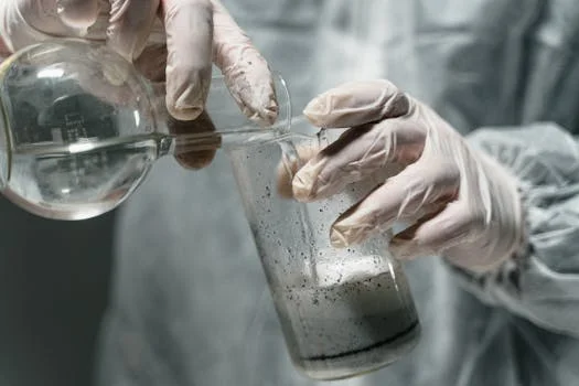
Step 1: Visual Inspection and Basic Tests
Start with a 30-minute settle test to assess particle settleability. Observe the supernatant for color, odor, and clarity. The table below correlates visual cues with likely causes:
| Visual Cue | Likely Cause | Particle Size Range | Next Diagnostic Step |
|---|---|---|---|
| Milky white | Colloidal silica, calcium carbonate | 10–100 nm | Zeta potential measurement |
| Brown/red | Iron hydroxides, clay | 1–10 μm | Particle size analysis |
| Gray/black | Metal sulfides, activated carbon fines | 0.1–5 μm | Microscopic examination |
| Oily sheen | Emulsified FOG, lubricants | 0.1–10 μm | Jar test with demulsifiers |
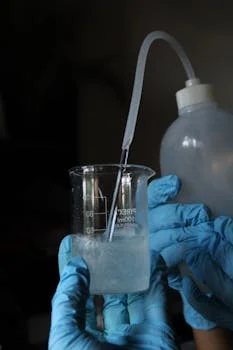
Step 2: Jar Testing for Coagulant/Flocculant Optimization
Jar tests simulate full-scale coagulation/flocculation to determine optimal chemical doses and pH. Follow this protocol:
- Fill six 1-L jars with wastewater samples.
- Adjust pH to target range (e.g., 6.0–7.5 for alum, 7.5–9.0 for ferric chloride).
- Add coagulant (e.g., alum, PAC) at varying doses (50–200 mg/L).
- Rapid mix at 200 rpm for 1 minute, then slow mix at 30 rpm for 10 minutes.
- Settle for 30 minutes and measure supernatant turbidity.
- Select the dose with the lowest turbidity and minimal sludge volume.
A metalworking plant may find that 120 mg/L PAC at pH 7.0 reduces turbidity from 600 NTU to 45 NTU, while overdosing to 180 mg/L increases sludge volume by 40%.
Step 3: Particle Size Analysis
Particle size distribution determines the most effective treatment technology. Use laser diffraction (0.1–2,000 μm) for broad ranges or dynamic light scattering (0.3 nm–10 μm) for colloids. Key insights:
- Particles <1 μm: Require coagulation/flocculation or membrane filtration.
- Particles 1–100 μm: Respond well to dissolved air flotation (DAF) or sedimentation.
- Particles >100 μm: Can be removed via screening or grit chambers.
Cost: $50–$200 per sample; turnaround: 24–48 hours.
Step 4: Zeta Potential Measurement
Zeta potential quantifies particle stability. Values <-30 mV or >+30 mV indicate stable suspensions; values between -10 and +10 mV suggest coagulation is likely. Typical ranges by industry:
- Textile: -40 to -60 mV (highly stable)
- Metalworking: -30 to -50 mV (moderately stable)
- Food processing: -20 to -40 mV (pH-dependent)
A textile plant with a zeta potential of -45 mV may require pH adjustment to 6.5 and cationic polymer addition to achieve coagulation.
Step 5: Microscopic Examination
Microscopy identifies biological and inorganic contaminants. Use 100–400x magnification to detect:
- Filamentous bacteria: Indicate sludge bulking (common in pulp/paper).
- Algae: Suggest nutrient overload (e.g., food/beverage).
- Metal oxides: Confirm corrosion or chemical precipitation.
Combine microscopy with particle size data to validate treatment selection. A pharmaceutical plant may find API crystals (5–20 μm) requiring microfiltration, while a food plant may identify yeast cells (5–10 μm) amenable to DAF.
For automated chemical dosing, explore our PLC-controlled dosing systems to streamline coagulation/flocculation.
Industrial Treatment Technologies: Matching the Solution to the Cause
Treatment technology selection depends on turbidity source, particle size, and effluent goals. The following comparison shows industrial-scale solutions:
| Technology | Best For | Removal Efficiency | Cost ($/m³) | Limitations | Key Parameters |
|---|---|---|---|---|---|
| Chemical Coagulation/Flocculation | Colloids, organic matter (50–1,000 NTU) | 70–95% | 0.20–0.80 | Sludge disposal, pH sensitivity | Optimal pH: 6.0–7.5 (alum), 7.5–9.0 (ferric); dosage: 50–200 mg/L |
| Dissolved Air Flotation (DAF) | FOG, emulsions, colloidal suspensions (100–2,000 NTU) | 90–98% | 0.50–1.50 | High energy use, microbubble fouling | Recycle ratio: 10–30%; air-to-solids ratio: 0.02–0.05; loading rate: 5–10 m³/m²·h |
| Membrane Bioreactors (MBR) | High-strength organics, near-reuse quality (<5,000 NTU) | 99% | 1.00–3.00 | Membrane fouling, high capital cost | Pore size: 0.04–0.4 μm; energy use: 0.5–1.5 kWh/m³; cleaning frequency: 1–3 months |
| Lamella Clarifiers | Settleable solids (100–1,000 NTU) | 60–85% | 0.30–0.70 | Low removal of colloids, sludge handling | Surface loading rate: 20–40 m³/m²·h; SVI target: <100 mL/g |
| Advanced Oxidation Processes (AOPs) | Recalcitrant organics (e.g., dyes, APIs) (200–1,000 NTU) | 80–95% | 1.50–4.00 | Byproduct formation (e.g., bromate), high chemical cost | Ozone dose: 5–15 mg/L; UV/H₂O₂: 10–30 mJ/cm² |
Chemical Coagulation/Flocculation
Coagulants like alum, ferric chloride, and polyaluminum chloride (PAC) neutralize particle charges, enabling aggregation. Dosage depends on turbidity level:
- 50–100 NTU: 50–100 mg/L alum
- 100–500 NTU: 100–150 mg/L PAC
- >500 NTU: 150–200 mg/L ferric chloride + polymer
Cost: $0.20–$0.80/m³. Limitations include sludge generation (0.5–1.5 kg/m³) and pH sensitivity (e.g., alum requires pH 6.0–7.5).
Dissolved Air Flotation (DAF)
DAF excels at removing FOG, emulsions, and colloidal suspensions. Microbubbles (30–50 μm) attach to particles, floating them to the surface for skimming. Key parameters:
- Recycle ratio: 20% (typical for textile and food processing)
- Air-to-solids ratio: 0.03 (optimal for metalworking)
- Loading rate: 5–10 m³/m²·h (higher for pulp/paper)
Our ZSQ series DAF systems achieve 95% turbidity removal at capacities of 4–300 m³/h. Cost: $0.50–$1.50/m³. For energy efficiency comparisons, see our DAF energy guide.
Membrane Bioreactors (MBR)
MBRs combine biological treatment with ultrafiltration, producing near-reuse-quality effluent (<0.2 NTU). Flat-sheet membranes (0.04–0.4 μm) resist fouling better than hollow-fiber, but both require regular cleaning (e.g., sodium hypochlorite or citric acid). Energy use: 0.5–1.5 kWh/m³. Our integrated MBR systems suit pharmaceutical and textile plants with space constraints.
Case Study: Reducing Textile Effluent Turbidity from 1,200 NTU to <30 NTU
A textile plant in Bangladesh faced repeated compliance failures due to effluent turbidity averaging 1,200 NTU (500 mg/L TSS). The plant used reactive and disperse dyes that formed stable colloidal suspensions with zeta potentials of -45 mV. Initial attempts with alum coagulation (100 mg/L) reduced turbidity to 300 NTU—below discharge limits but still problematic.
Diagnosis
- Jar tests: Optimal pH 6.5 with 120 mg/L PAC + 1 mg/L cationic polymer.
- Particle size analysis: 80% of particles <50 μm (ideal for DAF).
- Microscopy: Dye aggregates and cellulose fibers confirmed.
Solution
The plant installed a two-stage DAF system (ZSQ-50) with these parameters:
- Stage 1: pH adjustment to 6.5 + PAC dosing (120 mg/L).
- Stage 2: Cationic polymer (1 mg/L) + DAF with 20% recycle ratio.
- Flow diagram: Influent → pH adjustment → rapid mix → DAF Stage 1 → DAF Stage 2 → effluent.
Results
- Turbidity: 1,200 NTU → 25 NTU (98% removal).
- TSS: 500 mg/L → 30 mg/L.
- Chemical cost: $0.45/m³.
- Energy use: 0.3 kWh/m³.
- ROI: 18 months (avoided fines + reduced sludge disposal costs).
Lessons Learned
- pH control (6.0–7.0) is critical for PAC performance.
- Cationic polymers outperform anionic for dye removal.
- Two-stage DAF improves removal efficiency by 15–20% compared to single-stage.
Proactive Monitoring: Preventing High Turbidity Before It Starts
Proactive monitoring prevents high turbidity, reducing compliance risks and operational expenses. Key strategies include:
Online Turbidity Sensors
Nephelometric sensors (0–1,000 NTU) work for most applications, while backscatter sensors (1,000–10,000 NTU) suit high-turbidity streams. Calibrate weekly for critical applications (e.g., reuse water) and monthly for industrial effluent using formazin standards. Cost: $2,000–$10,000 per sensor.
Automated Chemical Dosing
Feedback loops using turbidity sensors adjust coagulant/flocculant doses in real time. A food processing plant may program its PLC-controlled dosing system to increase PAC dose by 20% when turbidity exceeds 100 NTU. Benefits include:
- Chemical savings: 15–30% vs. fixed dosing.
- Compliance: Reduces NTU spikes by 50–70%.
- Sludge reduction: Minimizes overdosing.
SCADA Integration
SCADA systems provide real-time turbidity trends and alarms. Set up alerts for:
- Turbidity >50 NTU for 15 minutes (warning).
- Turbidity >100 NTU for 5 minutes (critical).
Sample dashboard layout:
- Trend graph: Turbidity vs. time (24-hour window).
- Alert log: Timestamped NTU spikes with root cause notes.
- Chemical usage: Coagulant/flocculant consumption vs. turbidity.
For SCADA implementation guidance, see our cost guide for small plants.
Predictive Maintenance
Turbidity trends help schedule maintenance before failures occur. Examples:
- DAF systems: Clean skimmers when turbidity removal drops by 10%.
- MBRs: Schedule membrane cleaning when turbidity exceeds 0.5 NTU.
- Sedimentation tanks: Adjust sludge withdrawal when SVI >150 mL/g.
Predictive maintenance reduces chemical use by 30% and extends equipment life by 20–40%.
Frequently Asked Questions
What is the difference between turbidity and total suspended solids (TSS)?
Turbidity measures light scattering by suspended particles (NTU), while TSS measures particle mass (mg/L). The correlation varies by particle type:
- Clay: 1 NTU ≈ 1–2 mg/L TSS.
- Algae: 1 NTU ≈ 0.5 mg/L TSS.
- Metal oxides: 1 NTU ≈ 1.5 mg/L TSS.
TSS provides direct measurement, while turbidity offers an optical proxy. Both serve compliance purposes, but turbidity enables faster, more cost-effective real-time monitoring.
How do I choose between DAF and MBR for high turbidity?
Select DAF for FOG, emulsions, and colloidal suspensions (90–98% removal, $0.50–$1.50/m³). Choose MBR for high-strength organics and near-reuse quality (99% removal, $1.00–$3.00/m³). Consider:
- Influent turbidity: DAF <2,000 NTU; MBR <5,000 NTU.
- Space: DAF requires 20–30% less footprint than MBR.
- Operational complexity: MBR requires membrane cleaning; DAF requires skimmer maintenance.
What are the most common mistakes in turbidity treatment?
- Overdosing coagulants: Increases sludge volume by 30–50% and chemical costs. Validate with jar tests.
- Ignoring pH control: Reduces coagulation efficiency by 40–60%. Alum requires pH 6.0–7.5.
- Skipping diagnostics: Leads to 20–30% higher chemical costs. Particle size and zeta potential data guide technology selection.
- Poor mixing: Inadequate rapid mix (e.g., <200 rpm) reduces floc formation by 50%.
Can high turbidity affect downstream disinfection?
Turbidity >5 NTU reduces UV disinfection efficiency by 50–70% (EPA 2023 guidelines). Chlorine demand increases by 2–3 mg/L per 10 NTU. A plant with 30 NTU effluent may require 6–9 mg/L more chlorine than one with 2 NTU effluent. Aim for <2 NTU before disinfection to ensure pathogen inactivation.
How often should I calibrate my turbidity sensor?
Calibrate weekly for critical applications (e.g., drinking water reuse) and monthly for industrial effluent. Use formazin standards (0–1,000 NTU) and check for fouling. Clean sensors with 10% HCl or an ultrasonic bath every 1–3 months. Drift >10% indicates calibration failure or fouling.